
NumPy Core Syntax: Arrays, Indexing, and Quant Preprocessing
1. Basic Data Structures
The core data structure of NumPy is the ndarray (n-dimensional array). This is a multi-dimensional, homogeneous, and fixed-size array object.
To handle structured data, NumPy extends this with a data structure called a Structured Array.
It represents a record using a void type tuple, enabling NumPy to express record-type data. Consequently, there are primarily two array-related data types in NumPy.
1. Basic Data Structures
The first type is widely known, and we will use it to introduce most NumPy operations. The second type is also frequently used in quantitative finance. For instance, market data obtained via JoinQuant’s jqdatasdk allows returning this data type, offering significant convenience in storage and access compared to DataFrame. We will dedicate a separate section to this later.
Before using NumPy, we must install and import the library:
# 安装 NUMPY
pip install numpyTypically, we import and use NumPy using the alias np:
import numpy as npTo make result outputs more prominent when running these examples in a Notebook, we first define a cprint function. It outputs prompt messages verbatim but renders variable values in red font to distinguish them:
from termcolor import colored
def cprint(formatter: str, *args):
colorful = [colored(f"{item}", 'red') for item in args]
print(formatter.format(*colorful))
# 测试一下 CPRINT
cprint("这是提示信息,后接红色字体输出的变量值:{}", "hello!")Next, we will introduce basic CRUD (Create, Read, Update, Delete) operations.
1.1. Creating Arrays
1.1.1. Creating from Python Lists
We can create a simple array using the np.array syntax. In this syntax, we can provide a Python list or any object with an Iterable interface, such as a tuple.
arr = np.array([1, 2, 3])
cprint("create a simple numpy array: {}", arr)1.1.2. Pre-built Special Arrays
Often, we want NumPy to create arrays with specific values. NumPy provides this support, for example:
| Function | Description |
|---|---|
zeroszeros_like |
Creates an array of all zeros. zeros_like accepts another array and generates a zeros array with the same shape and dtype. Commonly used for initialization. Other _like functions follow this pattern. |
onesones_like |
Creates an array of all ones. |
fullfull_like |
Creates an array where all elements are filled with n. |
emptyempty_like |
Creates an empty array. |
eyeidentity |
Creates an identity matrix. |
random.random |
Creates a random array. |
random.normal |
Creates a random array following a normal distribution. |
random.dirichlet |
Creates a random array following a Dirichlet distribution. |
arange |
Creates an incrementing array. |
linspace |
Creates a linearly spaced array. Unlike arange, this method defaults to a closed interval. The interval between elements can be a float. |
# 创建特殊类型的数组
cprint("全 0 数组:\n{}", np.zeros(3))
cprint("全 1 数组:\n{}", np.ones((2, 3)))
cprint("单位矩阵:\n{}", np.eye(3))
cprint("由数字 5 填充的矩阵:\n{}", np.full((3,2), 5))
cprint("空矩阵:\n{}", np.empty((2, 3)))
cprint("随机矩阵:\n{}",np.random.random(10))
cprint("正态分布的数组:\n{}",np.random.normal(10))
cprint("狄利克雷分布的数组:\n{}",np.random.dirichlet(np.ones(10)))
cprint("顺序增长的数组:\n{}", np.arange(10))
cprint("线性增长数组:\n{}", np.linspace(0, 2, 9))warning
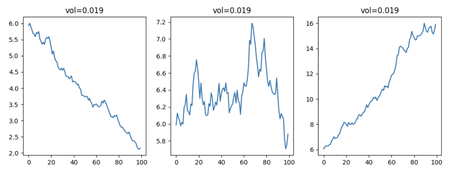
Although the name `empty` suggests it should generate an empty array, the generated array actually contains values. These values are neither `np.nan` nor `None`, but random values. Before using an array generated by `empty`, you must initialize it to handle these random values.Generating normal distribution arrays is very useful. In research, we often need to generate price sequences that satisfy certain conditions to further study and compare their characteristics.
For example, if we want to study certain indicators under upward and downward trends, we need the ability to first construct price sequences that conform to these trends. The following example demonstrates how to generate such sequences and plot them:
import numpy as np
import matplotlib.pyplot as pltreturns = np.random.normal(0, 0.02, size=100)
fig, axes = plt.subplots(1, 3, figsize=(12,4))
c0 = np.random.randint(5, 50)
for i, alpha in enumerate((-0.01, 0, 0.01)):
r = returns + alpha
close = np.cumprod(1 + r) * c0
axes[i].plot(close)The plotted graph is as follows:
The example also mentions Dirichlet distribution arrays. These arrays have a characteristic where the sum of all their elements equals 1. For example, in the efficient frontier optimization of Modern Portfolio Theory (MPT), we first need to initialize the weights of various assets (random values) and satisfy the constraint that the sum of asset weights equals 1 (obviously!). In this case, we can use the Dirichlet[2] distribution.
1.1.3. Converting from Existing Arrays
We can also create new arrays from existing ones through copying, slicing, repeating, etc.:
# 复制一个数组
cprint("通过 np.copy 创建:{}", np.copy(np.arange(5)))
# 复制数组的另一种方法
cprint("通过 arr.copy: {}", np.arange(5).copy())
# 使用切片,提取原数组的一部分
cprint("通过切片:{}", np.arange(5)[:2])# 合并两个数组
arr = np.concatenate((np.arange(3), np.arange(2)))
cprint("通过 concatenate 合并:{}", arr)
# 重复一个数组
arr = np.repeat(np.arange(3), 2)
cprint("通过 repeat 重复原数组:{}", arr)
# 重复一个数组,注意与 NP.REPEAT 的差异
# NP.TILE 的语义类似于 PYTHON 的 LIST 乘法
arr = np.tile(np.arange(3), 2)
cprint("通过 tile 重复原数组:{}", arr)question
What is the difference between `np.copy` and `arr.copy`? Are there other similar function pairs in NumPy, and what is the pattern?Note the role of the axis parameter in the concatenate function:
arr = np.arange(6).reshape((3,2))
# 在 ROW 方向上拼接,相当于增加行,默认行为
cprint("按 axis=0 拼接:\n{}", np.concatenate((arr, arr), axis=0))
# 在 COL 方向上拼接,相当于扩展列
cprint("按 axis=1 拼接:\n{}", np.concatenate((arr, arr), axis=1))1.2. Adding/Deleting and Modifying Elements
NumPy arrays are of fixed size. Generally, we do not recommend frequently adding or deleting elements from arrays.
However, if such a need arises, we can use the following methods to achieve addition or deletion:
| Function | Description |
|---|---|
append |
Adds values to the end of arr. |
insert |
Inserts the value value (scalar or array) at the position specified by obj (index or slice). |
delete |
Deletes elements at specified indices. |
Examples are as follows:
arr = np.arange(6).reshape((3,2))
np.append(arr, [[7,8]], axis=0)
cprint("指定在行的方向上操作、n{}", arr)arr = np.arange(6).reshape((3,2))
arr = np.insert(arr.reshape((3,2)), 1, -10)
cprint("不指定 axis,数组被扁平化:\n{}", arr)
arr = np.arange(6).reshape((3,2))
arr = np.insert(arr, 1, (-10, -10), axis=0)
cprint("np.insert:\n{}", arr)
arr = np.delete(arr, [1], axis=1)
cprint("deleting col 1:\n{}", arr)tip
Please definitely run the code here, especially the parts regarding `insert`, to understand what "flattening" means.Sometimes we need to modify the values of individual elements. This is how we do it:
arr = np.arange(6).reshape(2,3)
arr[0,2] = 3This involves how to locate an array element, which is the content of our next section.
1.3. Locating, Reading, and Searching
1.3.1. Indexing and Slicing
The indexing and slicing syntax in NumPy is roughly similar to Python, with the main difference being support for multi-dimensional arrays:
arr = np.arange(6).reshape((3,2))
cprint("原始数组:\n{}", arr)
# 切片语法
cprint("按行切片:{}", arr[1, :])
cprint("按列切片:{}", arr[:, -1])
cprint("逆排数组:\n {}", arr[: : -1])
# FANCY INDEXING
cprint("fancy index: 使用下标数组:\n {}", arr[[2, 1, 0]])
The above slicing syntax exists in Python but only supports one dimension. Therefore, similar operations on the following Python array will fail:
arr = np.arange(6).reshape((3,2)).tolist()
arr[1, :]The error提示 is list indices must be integers or slices, not tuple.
1.3.2. Finding, Filtering, and Replacing
In the previous section, we located array elements through indexing. However, in many cases, we first need to find the indices that meet specific conditions through conditional operations. This section introduces related methods.
| Function | Description |
|---|---|
np.searchsorted |
Searches for a specified value in a sorted array and returns the index. |
np.nonzero |
Returns the indices of non-zero elements, used to find elements in an array that meet conditions. |
np.flatnonzero |
Same as nonzero, but returns the indices of non-zero elements in the flattened version of the input array. |
np.argwhere |
Returns the indices of elements that meet conditions, equivalent to the transpose of nonzero. |
np.argmin |
Returns the index of the minimum element in the array (note: not the minimum index that meets a condition). |
np.argmax |
Returns the index of the maximum element in the array. |
# 查找
arr = [0, 2, 2, 2, 3]
pos = np.searchsorted(arr, 2, 'right')
cprint("在数组 {} 中寻找等于 2 的位置,返回 {}, 数值是 {}",
arr, pos, arr[pos - 1])
arr = np.arange(6).reshape((2, 3))
cprint("arr[arr > 1]: {}", arr[arr > 1])
# NONZERO 的用法
mask = np.nonzero(arr > 1)cprint("nonzero 返回结果是:{}", mask)
cprint("筛选后的数组是:{}", arr[mask])
# ARGWHERE 的用法
mask = np.argwhere(arr > 1)
cprint("argwere 返回的结果是:{}", mask)
# 多维数组不能直接使用 ARGWHERE 结果来筛选
# 下面的语句不能得到正确结果,一般会出现 INDEXERROR
arr[mask]
# 但对一维数组筛选我们可以用:
arr = np.arange(6)
mask = np.argwhere(arr > 1)
arr[mask.flatten()[0]]
# 寻找最大值的索引
arr = [1, 2, 2, 1, 0]
cprint("最大值索引是:{}", np.argmax(arr))When using searchsorted, note that the array itself must be sorted; otherwise, it will not yield correct results.
Lines 10–21 show how to find data in an array that meets conditions and return their indices.
The return value of argwhere is equivalent to the transpose of nonzero. In the case of multi-dimensional arrays, it cannot be directly used as an array index. Please compare the usage of nonzero and argwhere yourself.
In quantitative finance, there are many situations requiring filtering functionality. For example, when calculating upper shadow lines, we use the formula $(high - max(open, close))/(high - low)$.
If we want to calculate the upper shadow lines for the past $n$ periods all at once without using loops, we must use filtering functions like np.where and np.select.
The following example shows how to use np.select to calculate upper shadow lines:
import pandas as pd
import numpy as np
bars = pd.DataFrame({
"open": [10, 10.2, 10.1],
"high": [11, 10.5, 9.3],
"low": [9.8, 9.8, 9.25],
"close": [10.1, 10.2, 10.05]
})
max_oc = np.select([bars.close > bars.open,
bars.close <= bars.open],
[bars.close, bars.open])
print(max_oc)
shadow = (bars.high - max_oc)/(bars.high - bars.low)
print(shadow)
np.where is a function similar to np.select, but it only accepts a single condition.
arr = np.arange(6)
cprint("np.where: {}", np.where(arr > 3, 3, arr))This code implements the functionality of clipping numbers above 3 to 3.
This functionality is called clip, a very common technique in factor preprocessing used to handle outliers.
However, it cannot perform two-sided clipping. At this point, np.select can do this. This is the main difference between np.where and np.select:
arr = np.arange(6)
cprint("np.select: {}", np.select([arr<2, arr>4], [2, 4], arr))The result is that in the generated array, values less than 2 are replaced with 2, values greater than 4 are replaced with 4, and others remain unchanged.
1.4. Inspecting Arrays
When we call other people's libraries, we often need to exchange data with them. This may lead to data format incompatibility issues. To be able to debug, we must master some methods for viewing NumPy array properties.
We first generate a simple array as follows, and then view its various properties:
arr = np.ones((3,2))
cprint("dtype is: {}", arr.dtype)
cprint("shape is: {}", arr.shape)
cprint("ndim is: {}", arr.ndim)
cprint("size is: {}", arr.size)
cprint("'len' is also available: {}", len(arr))
# DTYPE
dt = np.dtype('>i4')
cprint("byteorder is: {}", dt.byteorder)
cprint("name of the type is: {}", dt.name)
cprint('is ">i4" a np.int32?: {}', dt.type is np.int32)# 复杂的 DTYPE
complex = np.dtype([('name', 'U8'), ('score', 'f4')])
arr = np.array([('Aaron', 85), ('Zoe', 90)], dtype=complex)
cprint("A structured Array: {}", arr)
cprint("Dtype of structured array: {}", arr.dtype)Just as Python objects have their own data types, NumPy arrays have their own data types. We can view the data type of an array using arr.dtype.
From lines 3 to 6, we output the array's shape, ndim, size, and len properties, respectively. ndim tells us the dimension of the array. shape tells us the size of each dimension. shape itself is a tuple, and the size of this tuple is equal to ndim.
size, when called without arguments, returns the product of the values of the elements in shape. len returns the length of the first dimension.
2. Array Operations
In the previous examples, we have already seen some examples that change the array's shape. For example, to generate a $3 \times 2$ array, we first use np.arange(6) to generate a one-dimensional array, and then change its shape to $(2, 3)$.
Another example is using np.concatenate, which changes the rows or columns of the array.
2.1. Increasing Dimensions
We can change the dimension of an array using reshape, hstack, and vstack:
cprint("increase ndim with reshape:\n{}",
np.arange(6).reshape((3,2)))
# 将两个一维数组,堆叠为 2*3 的二维数组
cprint("createing from stack: {}",
np.vstack((np.arange(3), np.arange(4,7))))
# 将两个 (3,1)数组,堆叠为(3,2)数组
np.hstack((np.array([[1],[2],[3]]), np.array([[4], [5], [6]])))2.2. Decreasing Dimensions
We can decrease the dimension of an array through operations like ravel, flatten, reshape, and *split.
cprint("ravel: {}", arr.ravel())
cprint("flatten: {}", arr.flatten())
# RESHAPE 也可以用做扁平化
cprint("flatten by reshape: {}", arr.reshape(-1,))
# 使用 HSPLIT, VSPLIT 进行降维
x = np.arange(6).reshape((3, 2))
cprint("split:\n{}", np.hsplit(x, 2))
# RAVEL 与 FLATTEN 的区别:RAVEL 可以操作 PYTHON 的 LIST
np.ravel([[1,2,3],[4, 5, 6]])This introduces four methods. ravel and flatten are quite similar in usage. ravel behaves similarly to flatten, except that ravel is a function of np and can act on arrays of type ArrayLike.
Flattening through reshape is also a common operation. Additionally, the vsplit and hsplit functions are introduced, which do the opposite of vstack and hstack.
2.3. Transposition
Furthermore, transposing an array is also an example of such operations. For instance, earlier we mentioned that the result of np.argwhere is actually the transpose of np.nonzero. Let's verify this:
x = np.arange(6).reshape(2,3)
cprint("argwhere: {}", np.argwhere(x > 1))
# 我们再来看 NP.NONZERO 的转置
cprint("nonzero: {}", np.array(np.nonzero(x > 1)).T)The two output results are exactly the same. Here, we achieved transposition through .T, which is a syntax sugar. The formal function is transpose.
Of course, since the reshape function is extremely powerful, we can also use it to complete transposition:
cprint("transposing array from \n{} to \n{}",
np.arange(6).reshape((2,3)),
np.arange(6).reshape((3,2)))Dirichlet, a German mathematician. He made outstanding contributions to number theory, Fourier series theory, and other areas of mathematical analysis, and is considered one of the earliest mathematicians to provide the modern definition of a function and one of the founders of analytic number theory. Dirichlet arrays can serve as initial values in MPT solving.