
Best Day to Buy Stocks: Sharpe 22.5 on Friday!
In Lesson 12, we discussed how to expand factors (or strategies) across four dimensions: volume, price, time, and space. In the time dimension, we noted that buying at different points from Monday to Friday yields different returns. This article reveals which day offers the highest return.
The problem is defined as follows:
Assume we buy at the closing price on Monday, Tuesday, ..., Friday, hold for 1, 2, 3, 4, or 5 days, and sell at the closing price. We calculate the average return, cumulative return, and Sharpe ratio. We select the more representative CSI 1000 index as the underlying asset.
Fetching Market Data
df = pro.index_daily(**{
"ts_code": "000852.SH"
})
df.index = pd.to_datetime(df.trade_date)
df.sort_index(ascending=True, inplace=True)
df.tail(10)The data we obtain spans from January 4, 2005, to the most recent trading day. In November 2024, this yields approximately 4,800 records.
Let’s first look at its overall trend:
df.close.plot()
If we had bought and held since January 4, 2005, we would have achieved roughly a 5x return over 19 years. Remember this number.
Calculating Grouped Returns
Next, we calculate the returns for buying on different days and holding for various periods. There is a simple algorithm here: first, calculate the corresponding daily return for each holding period, then group by weekday to obtain the results.
First, we add a grouping flag to df:
# Add a column to df as a grouping flag
df["weekday"] = df.index.map(lambda x: x.weekday())
# Convert numbers to more readable weekday names
df["weekday"] = df.weekday.map({
0: "Monday",
1: "Tuesday",
2: "Wednesday",
3: "Thursday",
4: "Friday"
})
df = df[["close", "weekday"]]
df.tail()At this point, we obtain:
| close | weekday | |
|---|---|---|
| trade_date | ||
| 2024-11-11 | 6579.0054 | Monday |
| 2024-11-12 | 6491.9723 | Tuesday |
| 2024-11-13 | 6474.3941 | Wednesday |
| 2024-11-14 | 6272.1911 | Thursday |
| 2024-11-15 | 6125.5126 | Friday |
| 2024-11-18 | 5974.5576 | Monday |
| 2024-11-19 | 6130.2848 | Tuesday |
| 2024-11-20 | 6250.8029 | Wednesday |
| 2024-11-21 | 6262.1644 | Thursday |
| 2024-11-22 | 6030.4882 | Friday |
Next, we calculate the returns for each period.
for period in range(1, 6):
df[f"{period}D"] = df.close.pct_change(period).shift(-period)
df.tail(10)At this point, we obtain:
| close | weekday | 1D | 2D | 3D | 4D | 5D | |
|---|---|---|---|---|---|---|---|
| trade_date | |||||||
| 2024-11-11 | 6579.0054 | Monday | -0.013229 | -0.015901 | -0.046635 | -0.068930 | -0.091875 |
| 2024-11-12 | 6491.9723 | Tuesday | -0.002708 | -0.033854 | -0.056448 | -0.079701 | -0.055713 |
| 2024-11-13 | 6474.3941 | Wednesday | -0.031231 | -0.053886 | -0.077202 | -0.053149 | -0.034535 |
| 2024-11-14 | 6272.1911 | Thursday | -0.023386 | -0.047453 | -0.022625 | -0.003410 | -0.001599 |
| 2024-11-15 | 6125.5126 | Friday | -0.024644 | 0.000779 | 0.020454 | 0.022309 | -0.015513 |
| 2024-11-18 | 5974.5576 | Monday | 0.026065 | 0.046237 | 0.048139 | 0.009361 | NaN |
| 2024-11-19 | 6130.2848 | Tuesday | 0.019659 | 0.021513 | -0.016279 | NaN | NaN |
| 2024-11-20 | 6250.8029 | Wednesday | 0.001818 | -0.035246 | NaN | NaN | NaN |
| 2024-11-21 | 6262.1644 | Thursday | -0.036996 | NaN | NaN | NaN | NaN |
| 2024-11-22 | 6030.4882 | Friday | NaN | NaN | NaN | NaN | NaN |
Now, let’s calculate the cumulative returns when buying at different times:
def cum_weekday_returns(df, period):
return ((1 + df[f"{period}D"]).cumprod() - 1).reset_index(drop=True)
returns_1d = df.groupby('weekday').apply(lambda x: cum_weekday_returns(x, 1))
returns_1d.swaplevel().unstack().plot()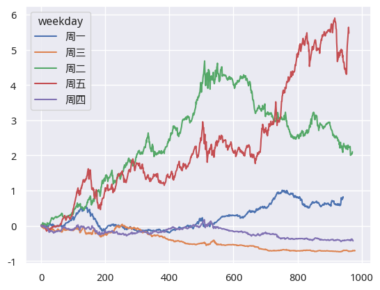
From the cumulative return chart, we can see that buying on Friday yields the highest return, approximately 5.47x. This result looks only slightly better than a simple buy-and-hold strategy. However, the capital occupancy is only 20% of that required for buy-and-hold. Therefore, if we calculate the annualized Alpha, it is significantly higher than buy-and-hold.
Of course, we have better metrics to evaluate the effectiveness of the Friday-buying strategy: the Sharpe ratio. Let’s first look at the Sharpe ratio for daily trading:
from empyrical import sharpe_ratio
sharpe_ratio(df.close.pct_change())The result we obtain is 0.46. Next, we calculate the Sharpe ratios for buying on different days from Monday to Friday:
for tm in ("Monday", "Tuesday", "Wednesday", "Thursday", "Friday"):
returns = returns_1d.swaplevel().unstack()[tm]
print(tm, f"{sharpe_ratio(returns):.1f}")The results show that buying on Tuesday even yields a higher Sharpe ratio. However, the Sharpe ratios for buying on Wednesday and Thursday are negative, which explains why the daily buy-in Sharpe ratio is not high.
The Ultimate Boss
Above, we only introduced the returns for buying on Friday and holding for one day. Considering that buying on Monday and Tuesday yields high Sharpe ratios, it is obvious that if we buy on Friday and hold for multiple days, the returns might be even higher. How many days should we hold to maximize returns, and how much higher will they be? It may exceed your imagination!
You may have read many articles and spent considerable time trying to replicate them, only to end up with nothing: either the code was incomplete, the data was inaccessible, or the article was fundamentally flawed. But we don’t want to give you such a negative experience. Like other articles on this platform, the conclusions in this article are replicable, and the data used is equally accessible to you. You can join my community and run/verify this article via the Quantide Research platform. If you verify its effectiveness, you can then copy the code to your local environment and incorporate it into your timing strategy. If the results cannot be verified, you can also leave the community.

def cum_weekday_returns(df, period):
return ((1 + df[f"{period}D"]).cumprod() - 1).reset_index(drop=True)
for period in range(1, 6):
returns = df.groupby('weekday').apply(lambda x: cum_weekday_returns(x, period))
returns.swaplevel().unstack().plot(title=f"Holding {period} Days")