
Quantide Weekly: Washout Detection via Numpy
This Week’s Highlights
- Ministry of Finance: China will intensify counter-cyclical fiscal policy adjustments.
- NBS Data: Industrial profits for listed enterprises fell 3.5% from January to September.
- NYSE: Plans to extend U.S. stock trading hours.
Next Week’s Focus
- Monday: On-site negotiations for the National Reimbursement Drug List begin.
- Thursday: National Bureau of Statistics releases October PMI data.
- U.S. Markets: The Q3 earnings season reaches its busiest week.
This Week’s Selection
- Series! Numpy Programming Essentials for Quants (8) – Violent Aesthetics: No Washout, No Rally. How to Detect Washout Patterns? (Application Case 5)
- Oct 25: The World Bank held the 110th meeting of its Development Committee. Liao Min, Vice Minister of Finance, stated that China will further intensify counter-cyclical fiscal policy adjustments. This includes implementing robust measures to resolve local government debt, stabilize the real estate market, increase incomes for key demographic groups, ensure livelihoods, and promote equipment upgrades and consumer goods trade-in programs. China remains confident in achieving a 5% growth target (Source: Ministry of Finance website).
- Jan–Sep: Total profits of industrial enterprises above designated size nationwide reached 522.816 billion RMB, a year-on-year decline of 3.5%.
- Today: The 2024 National Reimbursement Drug List on-site negotiations/bidding officially commenced. Staff from the National Healthcare Security Administration called in over ten companies, including China Resources Pharmaceutical, Baxter, Kangyuan Pharmaceutical, Kangzhe Pharmaceutical, Yichang Humanwell, and Zhida Tianqing, among others. The pace was noticeably faster than last year.
- BSE (Beijing Stock Exchange): Held special symposiums with brokers and listed companies. The BSE will promote the ability of enterprises to utilize M&A and restructuring tools, aiming to enhance the quality and investment value of BSE-listed companies.
- Central Huijin: Significantly increased holdings in broad-based ETFs in Q3. Just four CSI 300 ETFs and one ChinaAMC SSE 50 ETF consumed 300 billion RMB.
- NYSE: Plans to extend U.S. stock trading hours to 22 hours per business day.
Violent Aesthetics! No Washout, No Rally. How to Detect Washout Patterns?
No washout, no rally. During the chip accumulation phase, stock prices exhibit an upward trend, attracting many unstable followers. These followers become detrimental factors during the main upward phase.
Therefore, before the rally, the "main force" (market makers/institutional investors) employs a "washout" strategy to shake off these unstable, low-cost chips. This process often features extreme volatility, akin to a wild horse trying to throw off its rider.
Violent washouts can serve as one of the signals preceding a rapid market uptrend.
This article addresses the quantitative implementation: How can we rapidly detect washout patterns?
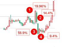
Violent washout is an empirical pattern observed in securities markets and lacks a strict definition. Generally, a pattern of "two bullish candles sandwiching one bearish candle" with significant price swings is considered a violent washout.
In this article, we define a violent washout as "two bullish candles sandwiching two bearish candles" with substantial price swings.
However, the method we introduce is fully applicable to other patterns, requiring only minor parameter adjustments.
As shown in the left chart, prior to position 1, the asset underwent a period of accumulation. Due to the price increase during this phase, some follower chips were attracted. At position 1, the main force pulled the price up by 20%. During this process, many follower chips were locked at the limit-up price.
Starting from Day 2, the main force began the washout, with consecutive daily declines of 14.4% and 18.9%. Chips bought at position 1, unable to withstand the massive drops, were sold at a loss. The main force increased its chip holdings and lowered its cost basis, creating room for the subsequent rally.
On Day 4, the main force pushed the stock up by 9.4%, signaling the end of the washout.
The subsequent consolidation days primarily served to allow time for new follower chips to discover the asset and gain confidence to buy. Following this, a series of small bullish candles established an upward trend, culminating in another 20% limit-up move. From Day 4, the short-term gain reached 87%.
Why did we define the washout using a 4-day pattern of "two bullish candles sandwiching two bearish candles"?
Because, in terms of time and space, a two-day washout yields better results (considering trader psychology: after a loss on Day 1, traders may not yet be desperate, but a continued drop on Day 2 makes them more likely to panic-sell). Additionally, from a technical indicator perspective, continuous sharp declines allow for adequate technical indicator repair, clearing space for the subsequent rally.
We set a threshold for price swings. If the swing of any bar during the period exceeds this threshold, we consider a washout to have occurred. In our example, the threshold is 0.05, representing a 5% swing.
Let’s look at the code implementation:
# Example 1
def feature_washout(bars, threshold=0.05):
"""Returns the position where the last washout ended in bars,
-1 indicates the last bar,
0 indicates no washout pattern exists.
"""
close = bars["close"]
opn = bars["open"]
truerange = np.maximum(np.abs(close[1:] - close[:-1]),
np.abs(opn-close)[1:])
# Convert to percentage
tr = truerange / close[:-1]
sign = (opn < close)[1:] * 2 - 1
signed_tr = tr * signWe used the variable name truerange because this code originates from the technical indicator TR.
This code solves the problem of converting price swings into a pattern represented by 1, -1, and 0, facilitating subsequent pattern retrieval.
If the daily swing exceeds 5%, or the body amplitude exceeds 5%, we mark it as 1 or -1; otherwise, it is marked as 0. The sign is determined by whether the candle is bearish (yin) or bullish (yang). Bearish candles are -1, and bullish candles are 1.
We implemented the calculation of bullish/bearish candles using this simple code:
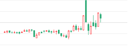
(opn < close) * 2 -1The result generates an array composed of 1s and -1s. Whether up or down, we always treat bearish candles as washouts. Thus, even if a high-open bearish candle closes up, we treat it as a washout.
The following image shows an example of a high-open bearish candle washout:
When judging whether the price swing or body amplitude of each bar exceeds the threshold, we use a simple trick: using np.maximum to select the maximum value from multiple arrays in an element-wise manner. That is, if there are arrays $A$ and $B$, then $np.maximum(A, B)$ returns an array where each element is the larger of the corresponding elements in $A$ and $B$.
In other words, if the result is $C$, then $C_0$ will be the larger of $A_0$ and $B_0$, $C_1$ will be the larger of $A_1$ and $B_1$, and so on.
Besides using the ufunc $np.maximum$, $np.max$ can also be used to accomplish this task, provided we first stack arrays $A$ and $B$ into a matrix:
# Example 2
A = np.arange(4)
B = np.arange(3, 7)
C = np.arange(8, 4, -1)
Z = np.vstack((A,B,C))
# Calculate column-wise maximum using np.max
r1 = np.max(Z, axis=0)
# Calculate maximum using np.maximum
r2 = np.maximum.reduce([A, B, C])
# Compare if results from both methods are identical
np.array_equal(r1, r2)To provide more information, the example demonstrates calculating the element-wise maximum for three arrays. The answer is to use the reduce method. If comparing only two arrays, np.maximum alone suffices.
After processing with Example 1, we might obtain an array as shown below:
[ ... 0.04 -0.02 -0.06 0.04 -0.04 -0.
Clearly, we should further binarize this into a pattern like [Big Yang, Big Yin, Big Yin, Big Yang] (i.e., [1, -1, -1, 1]):
# Example 3
encoded = np.select([signed_tr > threshold,
signed_tr < -threshold],
[1, -1], 0)
for i in range(len(encoded) - 3, 0, -1):
if np.array_equal([-1, -1, 1], encoded[i:i+3]):
return i - len(encoded) + 2
return 0We completed the binarization conversion using the select method. Next, we performed pattern matching via an inverse loop using array_equal.
In backtesting, we may need to extract all washout patterns from a long series of market data at once and test their effectiveness. The above code can also be optimized using numpy.lib.stride_tricks.sliding_window_view:
def feature_washout(bars):
...
washouts = []
for i, patten in enumerate(sliding_window_view(encoded, window_shape = 4)):
if np.array_equal(patten, [1, -1, -1, 1]):
washouts.append(i)
return washoutsBy binarizing price swings, we can conveniently match patterns later using array_equal. We do this because qualitative analysis is generally sufficient here: as long as the price swing exceeds 5%, whether it dropped 5.1% or 7.2%, we consider it a washout.
However, if you believe quantitative analysis still has value, you can also perform pattern matching using the Pearson correlation coefficient.