KS Test, Generalized Hyperbolic Fit, and Buying SSE Dip

In our last note, we asked a question: when the Shanghai Index plunges 4%, can you buy the dip? In this note, we'll use the K-S test to pin down the probability distribution of the Shanghai Index and answer that question. In a later note, we'll answer the same question with a different method.

K-S Test

Our first approach is to try our luck with the K-S test and see if Shanghai Index returns happen to match a known distribution. If we find one, we can easily use its cumulative distribution function (CDF) to compute the probability of further decline as:

$$ P = cdf(-0.04) $$

The K-S test is a non-parametric test in statistics. It can be used to test whether a sample comes from a given probability distribution (one-sample K-S test), or whether two samples share the same distribution (two-sample K-S test). The K-S test is named after its two proposers, the Russian statisticians Kolmogorov and Smirnov.

We can run the K-S test via scipy.stats.kstest. Its signature is:

1kstest(rvs, cdf, args=(), N=20, alternative='two-sided', method='auto')

Here rvs is the random variable sample — in our example below, we'll pass in 1,000 trading days of Shanghai Index returns. In the cdf argument, we pass the name of the candidate distribution to test.

It returns a KstestResult object, which includes key attributes such as statistic and pvalue.

Now let's run a one-sample test with kstest against each distribution implemented in scipy.stats to see if any of them pass:

12345pct = close[:-1]/close[1:] - 1
dist_names = ['burr12', 'dgamma', 'dweibull', 'fisk', 'genhyperbolic', 
              'genlogistic', 'gennorm', 'hypsecant', 'johnsonsu', 
              'laplace', 'laplace_asymmetric', 'logistic', 'loglaplace',
              'nct', 'norminvgauss']

12345678910111213141516xmin, xmax = min(pct), max(pct)
dist_pvalue = []

for name in dist_names:
    dist = getattr(scipy.stats, name)
    if getattr(dist, 'fit'):
        params = dist.fit(pct)
        ks = scipy.stats.kstest(pct, name, args=params)
        dist_pvalue.append(round(ks.pvalue, 2))
        
df = pd.DataFrame({
    "name": dist_names,
    "pvalue": dist_pvalue
})

df.sort_values("pvalue", ascending=False).transpose()

This gives the following output:

The figure may be too wide to read clearly on a phone. But all you need to know is that the first row, genhyperbolic — the generalized hyperbolic distribution — has the highest p-value, reaching 0.97.

Note that the p-value in scipy.stats.kstest may differ from what you understand as p-value elsewhere. Per its documentation and examples, a p-value greater than 0.95 means we accept the null hypothesis at 95% confidence: that rvs comes from the distribution indicated by the CDF.

The output therefore suggests that genhyperbolic, the generalized hyperbolic distribution, is the closest fit for the Shanghai Index among all candidates.

We can verify this conclusion visually:

1234567891011from scipy.stats import genhyperbolic

params = genhyperbolic.fit(pct)
rv = genhyperbolic(*params)

fig, ax = plt.subplots(1,1)
x = np.linspace(rv.ppf(0.01), rv.ppf(0.99), 100)
ax.plot(x, rv.pdf(x), label = 'genhyperbolic pdf', color="#EABFC7")

ax2 = ax.twinx()
_ = ax2.hist(pct, bins=50)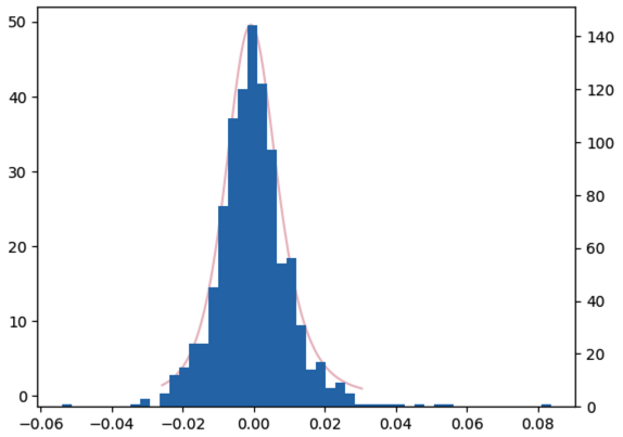

It's not just similar — it's virtually identical. The PDF curve neatly traces the outer contour of the empirical histogram.

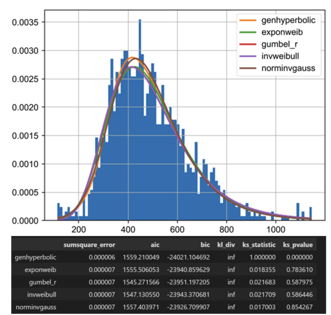
In fact, the Shanghai Index is not the only index that follows a generalized hyperbolic distribution. According to Souto's paper, Distribution Analysis of S&P 500 Financial Turbulence, published in Financial Mathematics (February 2023), the S&P 500 is also closest to this distribution.

12345from scipy.stats import genhyperbolic

params = genhyperbolic.fit(pct)
rv = genhyperbolic(*params)
print(f"继续下跌的概率为：{rv.cdf(-0.04):.2%}")

The result shows that the probability of further decline is only 0.16%. So, the conclusion is: this answer is based solely on historical data, for demonstrating quantitative methods only, and does not constitute any investment advice!