
HDBSCAN Clustering for Pairs Trading: 99x Speed Boost
Pairs trading is a trading strategy pioneered in the 1980s by Nunzio Tartaglia, a quantitative analyst at Morgan Stanley. Tartaglia is now the founder of Athena Asset Management in Italy. The strategy involves monitoring two securities that have historically exhibited strong correlation and tracking the price spread between them. Once the spread exceeds a certain threshold (e.g., $n$ standard deviations), mean reversion becomes highly probable. Traders then short the overpriced asset and go long on the underpriced one to capture profits.
 Nunzio Tartaglia
This strategy allows traders to profit in almost any market condition, making it a mainstream approach for large asset management firms.
For example, General Motors (GM) and Ford produce similar products (automobiles), so their stock prices tend to move similarly based on the broader automotive market. If GM’s stock price rises significantly while Ford’s remains unchanged, a trader employing a hedging strategy would sell GM stock and buy Ford stock. Assuming prices revert to their historical equilibrium: if GM’s price falls, the investor profits; if Ford’s price rises, the investor also profits.

The logic and effectiveness of this strategy are undeniable, resembling a mathematical theorem in its perfection. However, how do we find such paired assets?
Naturally, leading companies in the same industry often exhibit such relationships. However, because arbitrage opportunities in these areas are widely known, market efficiency tends to compress these spreads. For instance, if you executed a pairs trading strategy on China Construction Bank and Industrial and Commercial Bank of China over the past few years, the annualized return would likely not exceed 1%.
Moreover, a company’s business model is constantly evolving. Enterprises that once competed homogeneously may suddenly cease to be peers due to acquisitions or new business ventures. Old tracks may also see new predators enter. History repeats itself, yet it also opens new possibilities.
As quants, can we rely purely on data analysis to find these new opportunities more敏锐ly and quickly?
The answer is yes: we can discover potential paired assets solely based on asset price movements through cointegration tests.
Cointegration and Stationarity
How should we describe the relationship between GM and Ford using mathematical language? In mathematics (more precisely, statistics), this relationship is called a cointegration relationship.
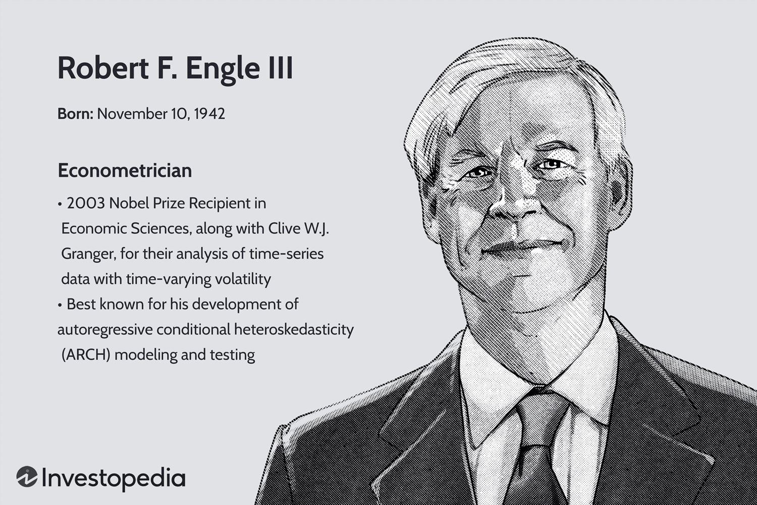
How do we test for cointegration? Engle and Granger proposed a two-step cointegration test in 1987: first, perform an OLS regression on two variables $X$ and $Y$, and then use the ADF test to check if $X$ and $Y$ are stationary. They won the 2003 Nobel Prize in Economics for their pioneering work in cointegration theory.
This brings us to another concept: stationary time series and stationarity tests.
A stationary time series is one where the statistical properties of random variables (such as mean, variance, autocovariance, etc.) remain constant over time. For example, white noise is a stationary time series with constant mean and variance. The figure below compares a stationary time series (top left) with several non-stationary time series:
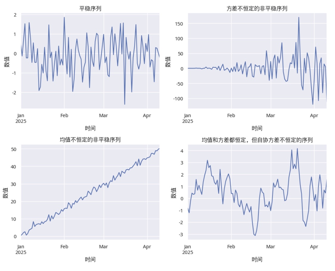
Obviously, for quants, stationary time series have very interesting properties: since a stationary time series has a constant mean, constant variance, and autocorrelation characteristics, once it deviates from the mean, it will eventually revert to the mean; otherwise, it would not be a stationary time series.
Thus, based on the assumption that a time series was stationary in the past and present, and will remain stationary in the future, we gain a rare ability to predict the future!
To test whether a time series is stationary, we generally use the Dickey-Fuller test.

For quants, asset price series and return series are two common types of time series. We can use the Dickey-Fuller test to determine if they are stationary:
import numpy as np
import pandas as pd
import matplotlib.pyplot as plt
from statsmodels.tsa.stattools import adfuller
start = datetime.date(2023, 1, 1)
end = datetime.date(2023, 12, 30)
barss = load_bars(start, end, ('000001.XSHE',))
close = barss.xs("000001.XSHE", level=1).close
returns = close.diff().dropna()
# 绘制平稳时间序列
plt.figure(figsize=(12, 6))
ax1 = plt.gca()
ax1.plot(close, label='Price')
ax1.grid(False)
ax2 = ax1.twinx()
ax2.plot(returns, label="Returns", color='orange')
ax2.grid(False)
lines, labels = ax1.get_legend_handles_labels()
lines2, labels2 = ax2.get_legend_handles_labels()
ax1.legend(lines + lines2, labels + labels2, loc='best')
plt.show()
# 进行 ADF 检验
result1 = adfuller(close)
result2 = adfuller(returns)
df = pd.DataFrame({
"ADF Stat": (result1[0], result2[0]),
"P-Value": (result1[1], result2[1]),
"Critical Values 1%": (result1[4]["1%"], result2[4]["1%"]),
"Critical Values 5%": (result1[4]["5%"], result2[4]["5%"]),
"Critical Values 10%": (result1[4]["10%"], result2[4]["10%"]),
}, index=["close", "returns"])
df.T
The code above produces the following results:
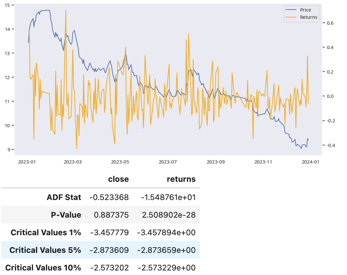
Stationarity testing is the second step of cointegration testing. The first step involves regressing two correlated time series to construct a residual series.
import statsmodels.api as sm
from statsmodels.tsa.stattools import adfuller
start = datetime.date(2021, 1, 1)
end = datetime.date(2023, 12, 30)
gsyh = "601398.XSHG"
jsyh = "601939.XSHG"
barss = load_bars(start, end, (gsyh, jsyh))
pair1 = barss.xs(gsyh, level=1).close
pair2 = barss.xs(jsyh, level=1).close
def hedge_ratio(price1: NDArray, price2: NDArray) -> float:
X = sm.add_constant(price1)
model = sm.OLS(price2, X).fit()
return model.params[1]
hr = hedge_ratio(pair1, pair2)
print(f"hedge_ratio 为:{hr:.2f}")
spreads = pair2 - pair1 * hr
result = adfuller(spreads)
if result[1] < 0.05:
print(f"p-value: {result[1]:.2f} < 0.05, 协整关系成立")
else:
print(f"p-value: {result[1]:.2f} > 0.05 协整关系不成立")This code completes a cointegration test. Moreover, it calculates the hedge ratio between the two price series. It is precisely through the hedge ratio that we can construct a stationary price spread series.
However, after understanding the principles, we generally do not use the above method for cointegration testing because statsmodels has already completed all this work for us:
from statsmodels.tsa.stattools import coint
result = coint(pair1, pair2)
t, p_value, *_ = resultAs long as the p-value is less than 0.05, we can consider the two time series to be cointegrated.
Performance Issues
Since cointegration testing is so straightforward, isn’t finding pairs trading opportunities a breeze? Not at all!
In a pool of assets, the computational load for finding cointegrated pairs is combinatorial. If the asset pool contains 100 assets, the number of calculations would be 4,950. If we limit the asset pool to domestic assets, considering that cointegration relationships may occur between China A-shares, funds, futures, and indices, the total number of assets could be around 10,000. This increases the computational load to nearly 50 million tests. This volume is enormous.
In our course environment, running 30,000 cointegration tests takes about 20 minutes, meaning each test takes approximately 40 milliseconds. Therefore, completing nearly 50 million cointegration tests would take roughly 24 days: by the time you finish calculating, the small insects living in your bathroom pipes—the Asian house mosquito (Clogmia albipunctata)—will have completed their entire life cycle.

At this point, clustering algorithms can exert their tremendous power: if we can divide these assets into several clusters and perform cointegration tests only within clusters, we can significantly reduce the number of cointegration tests.
Suppose we can cluster the samples into $K$ clusters, with the number of samples in each cluster being $( N_1, N_2, \ldots, N_K )$, where $( \sum_{i=1}^{K} N_i = N )$.
Then, the total number of cointegration tests is:
$$\sum_{i=1}^{K} \binom{N_i}{2} = \sum_{i=1}^{K} \frac{N_i (N_i - 1)}{2}$$
If the sample size in each cluster is roughly equal, the total number of cointegration tests will be much smaller. For example, if there are 100 assets, they can be clustered into 10 clusters of equal size. The total number of cointegration tests would then be $10 \times C_{10}^2$, i.e., 450 tests, a reduction of over 90% from the previous 4,950 tests.
HDBSCAN Clustering
There are many clustering algorithms; sklearn mentions over 10. However, for general-purpose use, the best clustering algorithm is likely HDBSCAN. It is not only fast (second only to K-Means) but also tolerant of noise, and its hyperparameters are easy to understand and set.
The figure below compares the clustering effects of HDBSCAN, DBSCAN, and K-Means on the same dataset:
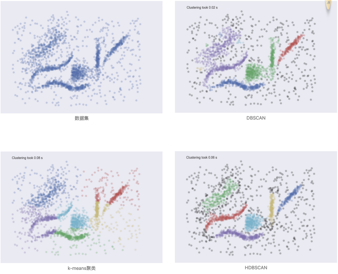
DBSCAN cannot find clusters sparser than the specified core density; K-Means assigns noise to the nearest cluster, and you must specify the number of clusters in the dataset. HDBSCAN’s performance is nearly perfect.
Next, we will use HDBSCAN to cluster assets. After clustering, we will perform cointegration tests and visualize the final results.
import hdbscan
import pandas as pd
from sklearn.manifold import TSNE
import plotly.express as px
start = datetime.date(2022, 1, 1)
end = datetime.date(2023,12,31)
barss = load_bars(start, end, 2000)
closes = (barss["close"].unstack().
ffill().
dropna(axis=1, how='any'))# 使用 HDBSCAN 进行聚类
clusterer = hdbscan.HDBSCAN(min_cluster_size=3, min_samples=2)
cluster_labels = clusterer.fit_predict(closes.T)
# 将聚类结果添加到 DataFrame 中
clustered = closes.T.copy()
clustered['cluster'] = cluster_labels
# 剔除类别为-1 的点,这些是噪声,而不是一个类别
clustered = clustered[clustered['cluster'] != -1]
clustered_close = clustered.drop("cluster", axis=1)
# 使用 t-SNE 进行降维
tsne = TSNE(n_components=3, random_state=42)
tsne_results = tsne.fit_transform(clustered_close)
# 将 t-SNE 结果添加到 DataFrame 中
reduced_tsne = pd.DataFrame(data=tsne_results,
columns=['tsne_1', 'tsne_2', 'tsne_3'],
index=clustered_close.index)
reduced_tsne['cluster'] = clustered['cluster']
fig_tsne = px.scatter_3d(
reduced_tsne,
x='tsne_1', y='tsne_2', z='tsne_3',
color='cluster',
title='t-SNE Clustering of Stock Returns',
labels={'tsne_1': 't-SNE Component 1',
'tsne_2': 't-SNE Component 2'}
)
fig_tsne.layout.width = 1200
fig_tsne.layout.height = 1100
fig_tsne.show()We will obtain a 3D t-SNE plot, where colors represent the clustering of each point. On our research platform, you can run the code to generate this 3D plot and drag it to change the viewing angle.
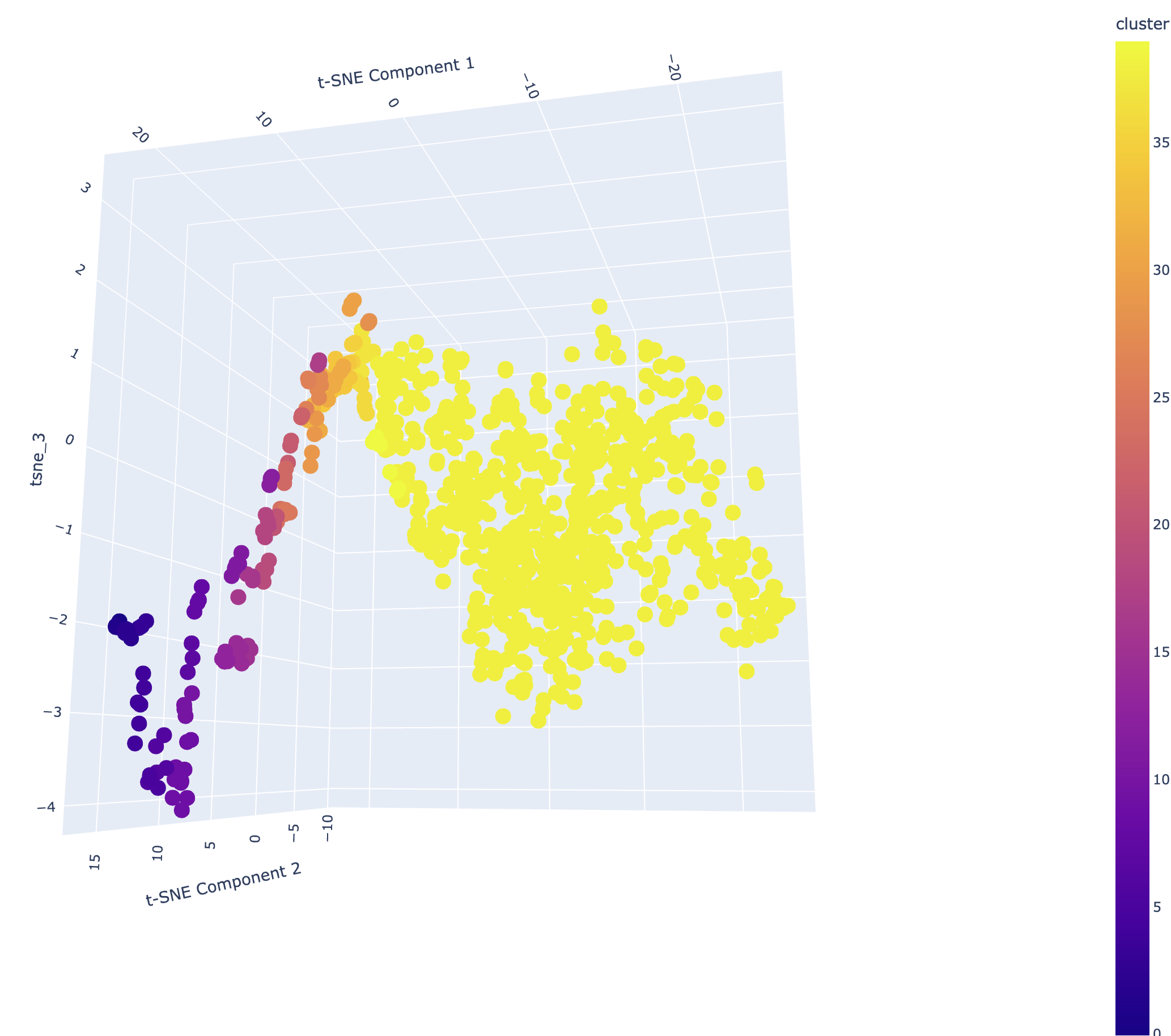
How effective is HDBSCAN’s clustering? Can we find cointegrated pairs within the categories it defines? We visualize the sample trends of the clusters and perform cointegration tests using the following code. This is the case for the randomly selected 12th cluster:
from statsmodels.tsa.stattools import coint
import hdbscan
import pandas as pd
from sklearn.manifold import TSNE
import plotly.express as px
start = datetime.date(2022, 1, 1)
end = datetime.date(2023,12,31)
barss = load_bars(start, end, 2000)
closes = barss["close"].unstack().ffill().dropna(axis=1, how='any')
# 使用 HDBSCAN 进行聚类
clusterer = hdbscan.HDBSCAN(min_cluster_size=3, min_samples=2)
cluster_labels = clusterer.fit_predict(closes.T)
clustered = closes.T.copy()
clustered['cluster'] = cluster_labels
# 剔除类别为-1 的点,这些是噪声,而不是一个类别
clustered = clustered[clustered['cluster'] != -1]
clustered_close = clustered.drop("cluster", axis=1)
plt.figure(figsize=(12,10))
cluster_12 = clustered.query("cluster == 12").index.tolist()
for code in cluster_12:
bars = barss.xs(code, level=1)["close"]
plt.plot(bars)
pairs = []for i in range(len(cluster_12)):
for j in range(i + 1, len(cluster_12)):
pair1 = cluster_12[i]
pair2 = cluster_12[j]
price1 = barss.xs(pair1, level=1)["close"].ffill().dropna()
price2 = barss.xs(pair2, level=1)["close"].ffill().dropna()
minlen = min(len(price1), len(price2))
t, p, *_ = coint(price1[-minlen:], price2[-minlen:])
if p < 0.05:
pairs.append((pair1, pair2))
row = max(1, len(pairs) // 3)
col = len(pairs) // row
if row * col < len(pairs):
row += 1
cells = row * col
fig, axes = plt.subplots(row, col, figsize=(col * 3,row * 3))
axes = np.array(axes).flatten()
fig.suptitle('Cointegrated Pairs')
plot_index = 0
for pair1, pair2 in pairs:
ax = axes[plot_index]
price1 = barss.xs(pair1, level=1)["close"]
price2 = barss.xs(pair2, level=1)["close"]
ax.plot(price1, label=pair1)
ax.plot(price2, label=pair2)
ax.set_title(f'{pair1[:-5]} & {pair2[:-5]}')
ax.set_xticks([])
plot_index += 1
plt.tight_layout()
plt.show()
print(len(pairs)/(len(cluster_12) * (len(cluster_12) - 1)) * 2)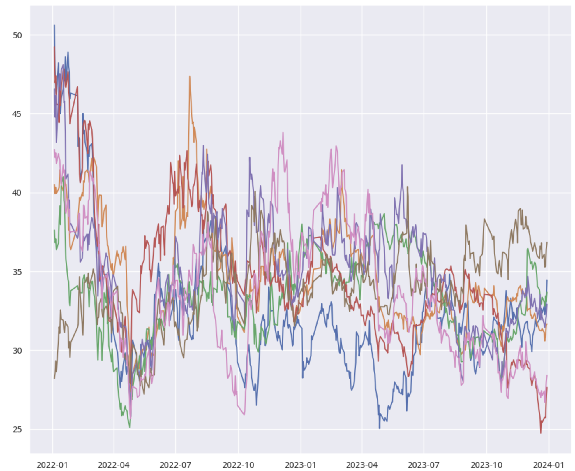
From the results, we can see that the individual stock trends within a cluster are almost identical, but not all combinations within the cluster are cointegrated pairs. This is easy to understand: clustering has its own logic, and cointegration has its own logic. There is overlapping space between them, but they are certainly not the same thing.
The important point is that we have significantly compressed the computation time. Time flies like an arrow, fire flashes like a stone, life is like a dream. But now, in this fleeting moment, we have discovered a new wealth code. Being first in quant is extremely important; once others find the opportunity, the limited capital capacity will be taken by them.
Help Wanted! Hurry Up and Recruit!

At Quantide, we research (quant framework development, trading strategies) and produce content (via our public account or video account), always growing, using the Feynman learning method. After all, quantitative research is like Sisyphus rolling the stone up the hill: there is no one-time success, only daily failures, learning, and starting over!
Specifically, this position has the following (desensitized) typical symptoms: proficiency in the probability and statistics knowledge required for quant work, mastery of Python, numpy, pandas, statsmodels, scipy, and machine learning algorithms, a love for writing, photo editing skills, understanding of AI, and a super fan of new concepts and technologies. A true hexagon warrior. However, whether you are a triangle or a square, as long as you truly love this work, you are welcome to apply. What I want most right now is a learning blogger, someone who genuinely learns, not just someone posing for photos.
For specific positions, please call hr@quantide.cn for inquiries, or directly send your resume. Students can apply for internship positions.

Passion is the best teacher. Waiting for you at the center of the universe.