Second-Derivative Momentum Factor: 61% Annualized Alpha on China A-Shares

In this episode, we introduce a second-derivative factor. We will demonstrate the exploration and optimization process for this factor, further explaining the principles of factor analysis, including:

1. How to configure Alphalens to use custom layers.
2. The mathematical principles behind the second-derivative momentum factor.
3. The distinction between "By quantiles" and "By bins" layering.

Finally, using a 40% sample of China A-shares, we determined that the optimal parameter for the second-derivative factor over the last six months is a 5-day window. Under this parameter, the annualized Alpha is 38.4% (long-short) and 61.5% (long-only), with a Beta of -0.12, indicating returns are independent of the market.

The table below shows the performance under different periods and long-short configurations:

Condition	Alpha	Beta	Cumulative Return
Long-Short, 2	30.6%	-0.06	15%
Long-Short, 4	35.3%	-0.1	17%
Long-Short, 5	38.4%	-0.12	19%
Long-Short, 6	37.3%	-0.12	18%
Long-Short, 8	32.4%	-0.06	14.8%
Long-Short, 10	23.2%	-0.07	11%
Long-Only, 10	17.6%	-0.60	15%
Long-Only, 5	61.5%	-0.58	37%

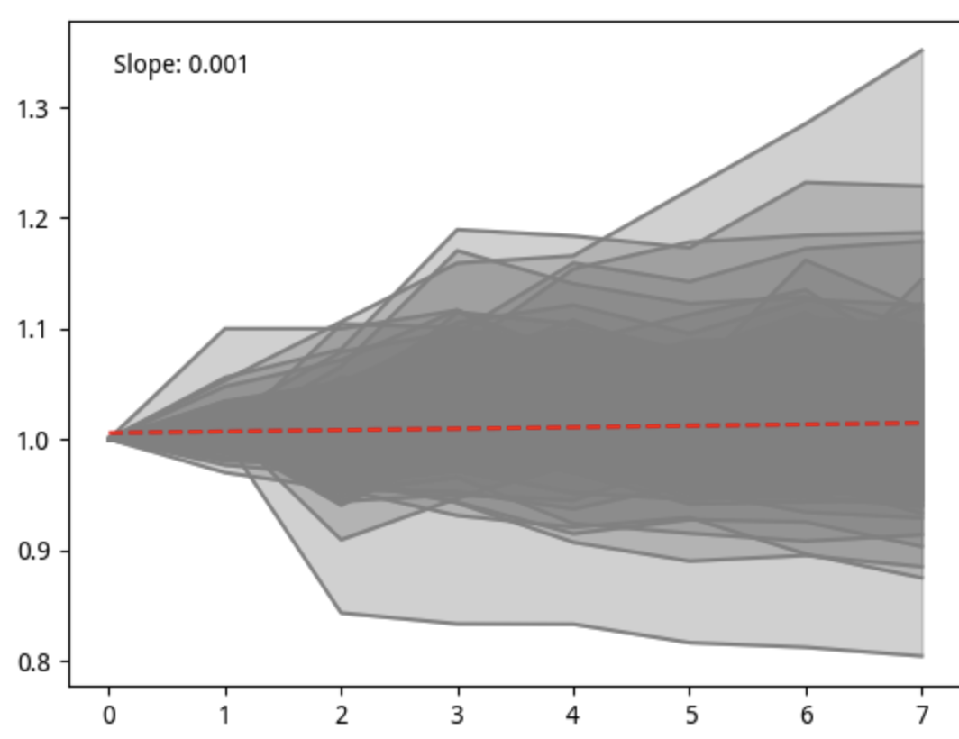
We randomly selected a sample from a single day, plotted its 7-day price trajectory, and fitted a trendline for the sample mean to verify the reliability of the factor analysis:

Upon purchasing this article, please send a private message to receive an online URL and login password. This provides access to all code, China A-share market data since 2005 (including minute-level data), and a backtest engine, supporting online execution and verification.

---

In the previous episode, we examined the slope factor. Essentially, the slope factor is a first-derivative momentum factor. For example, an array generated in the following manner has a slope and first derivative that are equal:

1234567891011121314from scipy.stats import linregress

slope = 0.2
x = np.arange(10)
y = slope * x + 1

d1 = np.diff(y).mean()

# If we calculate the slope via linear regression
alpha, beta, *_ = linregress(x, y)

print(f"slope is {slope:.1f}")
print(f"first derivative is {d1:.1f}")
print(f"slope by linear regression is {alpha:.1f}")

All three outputs are 0.2. If we use the second derivative of the price sequence as a factor, can it predict future trends? Let's look at the results first, then discuss the underlying principles.

Second-Derivative Momentum Factor Testing

1234567891011def d2_factor(close: NDArray, win: int = 10) -> NDArray:
    n = len(close)

    d1 = close[1:]/close[:-1] - 1
    d2 = d1[1:] - d1[:-1]

    factor = move_mean(d2, win)
    # Pad on the left to match the input length
    factor = np.pad(factor, (n-len(factor), 0), ...)
    
    return factor

---

The code above generates a second-derivative momentum factor. Note that we use close[1:]/close[:-1]-1 instead of the standard first derivative to achieve a form of normalization. If we did not do this, the factor for high-priced stocks would always be larger than that for low-priced stocks, resulting in permanently higher factor exposure.

The factor's parameter is win, representing the time window over which the second derivative is calculated.

We then use Alphalens for factor testing. For the first call to Alphalens, we layer by quantiles with 10 layers.

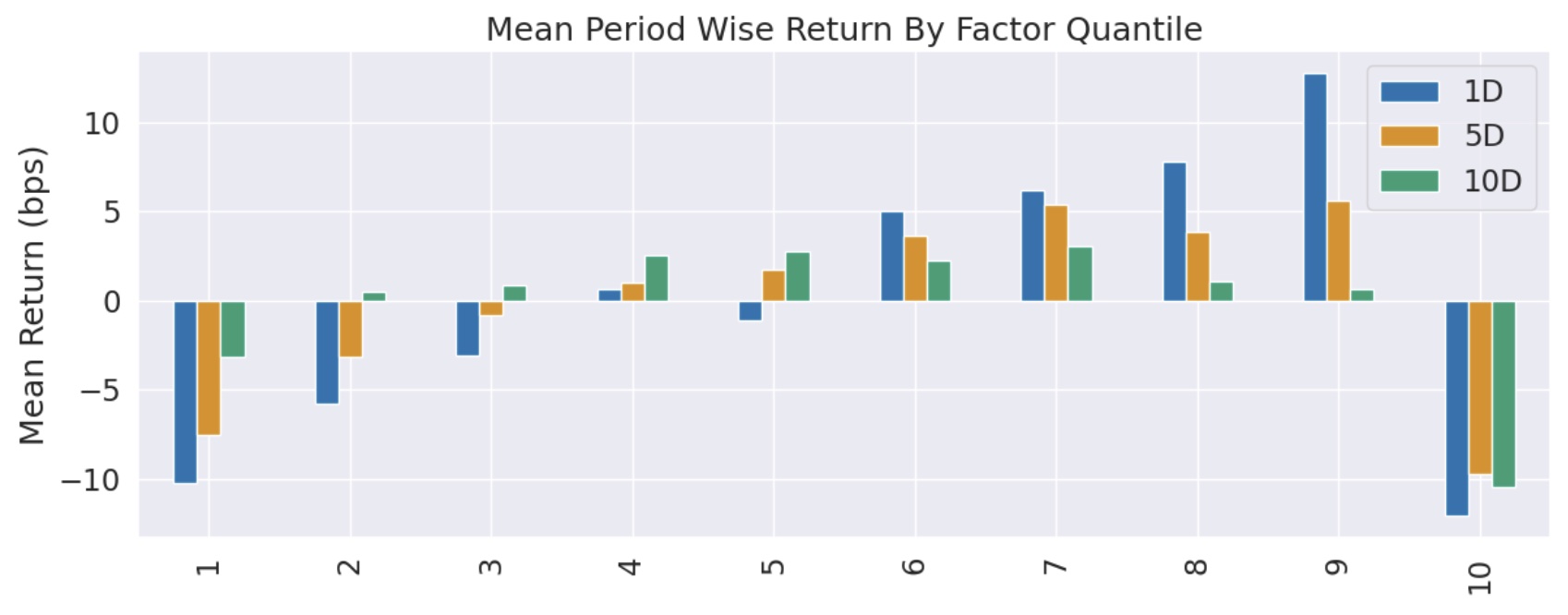
From the layering chart, it is clear that continuing with收益 analysis is meaningless; we must optimize first.

First Optimization

Considering that long returns peak at the 9th layer, we consider dropping the 10th layer to analyze the results.

When using Alphalens for analysis, there are generally three steps:

1. Construct the factor.
2. Preprocess data, typically by calling get_clean_factor_and_forward_returns.
3. Call create_full_tearsheet to execute factor testing and output reports. Its input is the output from step 2.

---

Alphalens performs layering in step 2. It then uses the output from step 2 as the input for step 3.

Therefore, after obtaining the output from step 2, we can drop the 10th layer and call create_full_tearsheet for收益 analysis. In this way, Alphalens sees the top layer as the 9th layer, and all analysis is based on this.

According to Alphalens' official documentation, this is allowed.

The output of step 2 is a DataFrame with the following format:

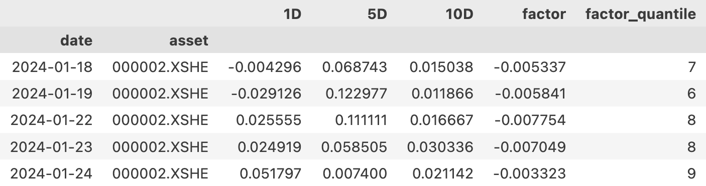
Thus, to drop the 10th layer, we can do the following:

1factor_data = factor_data[factor_data.factor_quantile <= 8]

This time, we obtained a satisfactory layering mean收益 chart: monotonic and increasing, fully suitable for further factor analysis.

---

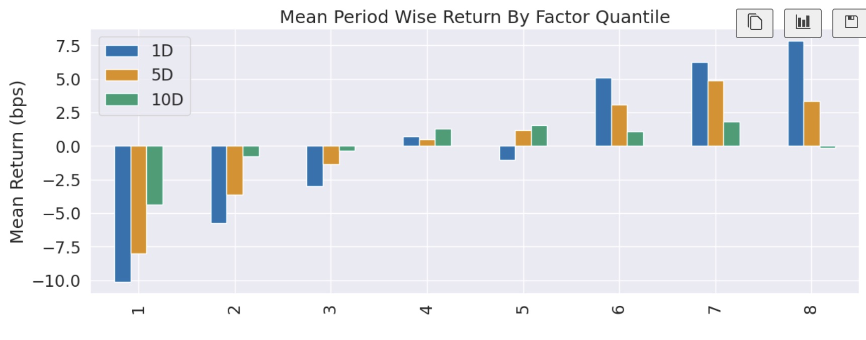
This chart is essentially a complete reproduction of the previous one, except for the missing 10th layer. However, the 9th layer is now the top layer, which is the layer Alphalens will go long on when calculating long-short returns.

The Alpha we now obtain is 23.2% (1-day annualized), Beta is -0.07, and the cumulative return over 7 months is approximately 11%.

Long-Only Scenario

In previous episodes, we discussed that due to regulatory factors, not everyone can short sell. So, let's look at the factor's performance in a long-only scenario.

This time, the annualized Alpha is only 17.6%, with a Beta of -0.6. However, the cumulative return over 7 months is around 15%, which is slightly higher.

---

Condition	Alpha	Beta	Cumulative Return
Long-Short, 10	23.2%	-0.07	11%
Long-Only, 10	17.6%	-0.60	15%

Comparing the cumulative return charts from both scenarios, we can see that while the absolute return of the long-short portfolio is lower, its risk-mitigation capability is stronger:

Long-Short Portfolio

Long-Only

---

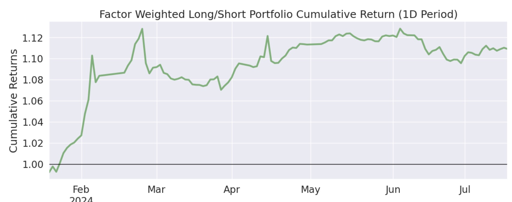
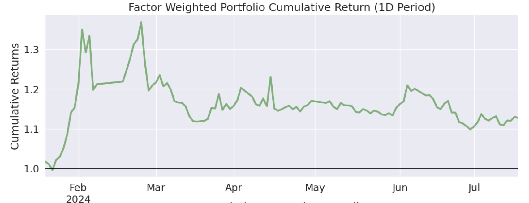
Why is the Alpha of the long-short portfolio higher than the long-only, yet its cumulative return is lower? This may be due to some negative effects during the shorting process of the second-derivative factor. Some strong stocks, after a sharp drop (where the second derivative is negative), often experience a small rebound. If we short right before this small rebound, it results in losses.

Finding the Most Effective Window

So far, we have used a 10-day window to calculate the second derivative. What if we use other windows? We tested data for 2, 4, 6, and 8 days. Now, let's summarize all the data:

Condition	Alpha	Beta	Cumulative Return
Long-Short, 2	30.6%	-0.06	15%
Long-Short, 4	35.3%	-0.1	17%
Long-Short, 5	38.4%	-0.12	19%
Long-Short, 6	37.3%	-0.12	18%
Long-Short, 8	32.4%	-0.06	14.8%
Long-Short, 10	23.2%	-0.07	11%
Long-Only, 10	17.6%	-0.60	15%
Long-Only, 5	61.5%	-0.58	37%

It appears that on the China A-share market, the second-derivative momentum factor performs best with a period of 5. At this point, if we can construct a long-short portfolio, the annualized Alpha is 38.4%, and the year-to-date cumulative return is 19%; if we can only construct a long-only portfolio, the annualized Alpha is 61.5%, and the year-to-date cumulative return is 37%.

A Review of High School Math

The slope factor (i.e., first-derivative factor) discussed in the previous episode reflects the speed of price increase.

So, what does the second-derivative factor represent?

---

The second-derivative factor reflects the acceleration of price changes. When the first derivative is positive but the second derivative is negative, prices will still rise, but the trend slows down, potentially signaling a trend reversal. The converse is also true. The following formula shows a function with a second derivative:

$$ y = a x^2 + b x + c $$

When $a$ and $b$ take values in $[-1, 0, 0, 1]$ and $[10, 10, -10, -10]$ respectively, we obtain the following graph:

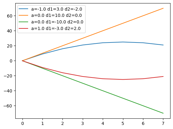
This graph illustrates that the second derivative has a corrective effect on the trend of security prices. A stock in an uptrend, if the second derivative remains negative, will eventually reach a peak and then turn downward; conversely, a stock in a downtrend, if the second derivative remains positive, will eventually hit a bottom and then turn upward.

Precisely because of this, unlike the first derivative, the second derivative has the ability to predict changes in price trends in advance. It is a form of reversal momentum.

In the tests, the best-performing parameter was 5 days. Considering that the second derivative requires two additional windows to calculate, we actually generate trading signals based on the past 7 days of data.

7 days, the number of God.

---

Seeing Is Believing

Seeing an Alpha of 38%, I must admit, was surprising.

Is it real? Or has some Pseudo-Logoi (the god of lies) sneaked in somewhere?

Although we can trust Alphalens as a guarantee of quality, you might prefer to trust your own keen eyes over a pile of statistical numbers.

Therefore, I decided to plot the price trajectories of individual stocks in the 9th layer. The plotting method is as follows: first, take all targets with quantile = 9 on a specific day (denoted as T0), then take the closing prices for the most recent 9 days (up to T0). Before plotting, normalize the starting point of the closing prices to 1.

In the plot, we used a total of 199 samples, which is sufficient for representativeness and robustness.

---

The red line in the graph is the trendline, with a slope of 0.001, indicating an overall upward trend; the color intensity represents the distribution density of the samples, showing that more are distributed above the zero line.

I like to draw inspiration from some stock market proverbs. Due to differences in company fundamentals, market mechanisms, and trading systems, directly copying overseas stock market practices does not work. The underlying nature of our market博弈 (game theory/competition) is heavier.

Logically, the stock market proverbs related to the second-derivative momentum factor are golden pits and圆弧 tops (rounding tops), or V-shaped reversals. So, can we intuitively plot how many beautiful "golden pits" exist among these targets?

It is difficult to draw them all in one chart with a single parameter: the cycle, depth, and construction phase of each golden pit vary. As the saying goes, "Huan Fei and Yan Shou" (beauty varies), it is hard to capture all the elegance in one stroke.

By bins, or By quantiles?

In this test, we have consistently used layering by quantiles, without exploring layering by bins.

By quantiles is a ranking-based layering. This is determined by the definition of quantiles. Using the by bins method, we focus more on the financial meaning of the factor value itself.

For example, for RSI, its value ranges from 0 to 100. It is generally believed that values above 80 are "overbought" and values below 20 are "oversold." Therefore, using the factor value directly is meaningful.

This article did not use the by quantiles method, partly because the signal significance of the factor value itself may not be strong:

We look for buy or sell signals by verifying whether the price goes up or down later. However, the second derivative only tells us the direction of the trend change, not the immediate rise or fall.

Therefore, we might be better off using its ranking for the factor, as capital often seeks targets with the strongest reversal momentum.

---

On the other hand, I am unclear about its minimum, maximum, and distribution, making it difficult to provide a bins array in practice. This is also the reason for not using by bins.

Of course, this is not absolute. Perhaps, if time permits, we should also explore layering by bins.