
PEPE’s Warning: How High Can the Market Go?
The market has been surging joyfully, but for the developers at Eastmoney, it might mean overtime. The rally is so strong that their programs are overflowing:
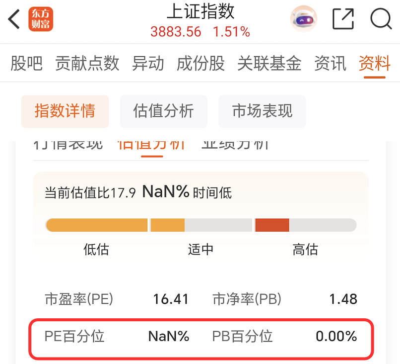
What’s going on here?
Reviewing the Basics
In September 2024, we published “A Heart-Stopping Scene Before the Holiday! Who Can Tell Me if A-Shares Are Undervalued?”. In that article, we used akshare to fetch the Shanghai Composite Index’s price-to-earnings (PE) ratio and conducted quantile and trend analysis to explore the valuation landscape of the A-share market at that time.
Our conclusion then was:
Based solely on quantile statistics, A-shares appear undervalued. However, considering the PE ratio’s persistent upward trend and the divergence between PE and index performance over the past year, it remains questionable to label A-shares as undervalued. More dimensions should be incorporated into the assessment.
It is now August 2025, nearly a year later. Judging by trading volume, the market seems to have entered a frenzy. Can the techniques we used last year still predict future trends?
Let the data speak.
Fetching Index PE Data via Tushare
Tushare gave us a break last week, but fortunately, it has since resumed operations. To obtain index PE data, we utilize the index_dailybasic function.
import pandas as pd
import matplotlib.pyplot as plt
import matplotlib.dates as mdates
from datetime import datetime
pro = pro_api()def get_index_pe_close(ts_code='000001.SH', start_date='20100101', end_date='20250825'):
# 获取指数PE数据
df_pe = pro.index_dailybasic(ts_code=ts_code,
start_date=start_date,
end_date=end_date,
fields='trade_date,pe_ttm')
df_pe.rename(columns={'trade_date': 'date', 'pe_ttm': 'pe'}, inplace=True)
df_pe['date'] = pd.to_datetime(df_pe['date'])
df_pe.set_index('date', inplace=True)
# 获取指数收盘价数据
df_price = pro.index_daily(ts_code=ts_code,
start_date=start_date,
end_date=end_date,
fields='trade_date,close')
df_price.rename(columns={'trade_date': 'date'}, inplace=True)
df_price['date'] = pd.to_datetime(df_price['date'])
df_price.set_index('date', inplace=True)
# 合并数据
df = df_pe.merge(df_price, left_index=True, right_index=True, how='inner')
# 排序
df.sort_index(inplace=True)
# 移除PE为空的记录
df = df.dropna(subset=['pe'])
return dfAfter obtaining the PE data, let’s first examine the intuitive trend:
# 绘制PE走势图
fig, ax = plt.subplots(figsize=(12,6))
color = "tab:red"
ax.plot(df.index, df["pe"], label="PE", color=color)
ax.set_xlabel("Year")
ax.set_ylabel("PE", color=color)
ax.xaxis.set_major_locator(mdates.YearLocator())
ax.xaxis.set_major_formatter(mdates.DateFormatter('%Y'))
df = get_index_pe_close(start_date="20100101")
# 添加分位数线
for i in range(1, 4):
quantile = df["pe"].quantile(i/4)
ax.axhline(quantile, color='gray', linestyle='--', label=f"{i/4:02.0%}")
plt.title("SSE Index PE Ratio (via Tushare)")
plt.legend(loc="upper left")
plt.grid(True)
plt.show()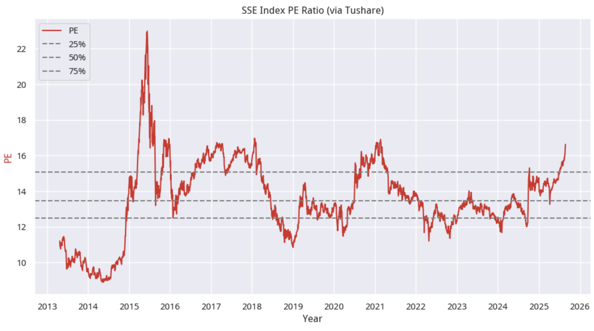
The data indicates that if we ignore the crazy history of 2015 (off-exchange margin financing with leverage), the current PE level is quite high.
Just how high?
def show_pe_quantile(df):
# 计算当前PE分位数
current_pe = df['pe'].iloc[-1]
rank = df['pe'].rank().iloc[-1]
percentile = rank / len(df)
print(f"当前PE分位: {percentile:.2%}")
show_pe_quantile(df)
df = df[df.index > '2016-01-01']
show_pe_quantile(df)If we calculate from 2013 (Tushare does not seem to have earlier data), the current PE quantile is 95.18%. If we calculate from January 2016, the current PE quantile has reached 98.81%, approaching perfection. For an index, this is indeed quite high.
What is the current PE value relative to historical highs? This can be easily calculated using pandas:
def find_days_since_max_pe(df):
"""计算当前的PE是过去多少天以来的最大值"""
if df.empty or len(df) < 2:
return None
# 获取当前PE值
current_pe = df['pe'].iloc[-1]
# 找到当前PE值在历史数据中的最大值位置
max_pe_idx = df['pe'].idxmax()
# 计算距离最大值日期的天数
current_date = df.index[-1]
days_since_max = (current_date - max_pe_idx).days
return days_since_max, max_pe_idx
find_days_since_max_pe(df)The answer is that the current PE value is the maximum since January 24, 2018, marking a new high for the past seven years.
Assuming the index stabilizes, the only way for the PE to return to a safe zone is through corporate profit growth. If the index remains at this level, how much must corporate profits increase for the PE to return to a safe zone?
We calculate this using the following method:
def required_earnings_growth(df, target_percentile=0.75, target_index=None):
"""计算使PE分位数降到目标值所需的盈利增长百分比"""
if df.empty:
return None
# 获取当前PE值和当前指数点位
current_pe = df['pe'].iloc[-1]
current_index = df['close'].iloc[-1]
# 如果指定了目标指数点位,则计算在该点位下的目标PE值;否则使用数据框中目标分位数对应的PE值
if target_index is not None:
# 根据PE = Price / Earnings,计算目标指数点位下的PE值
# 假设盈利不变,目标PE = target_index / (current_index / current_pe)
# 即 target_pe = target_index * current_pe / current_index
current_pe = target_index * current_pe / current_index
# 计算目标PE值(目标分位数对应的PE)
target_pe = df['pe'].quantile(target_percentile)
# 如果当前PE已经低于目标PE,则不需要盈利增长
if current_pe <= target_pe:
return 0.0
# 计算所需盈利增长百分比
# PE = Price / Earnings => Earnings = Price / PE
# 要使PE从current_pe降到target_pe,需要:
# (Price / target_pe) / (Price / current_pe) - 1 = current_pe / target_pe - 1
required_growth = (current_pe / target_pe) - 1
return required_growth
required_earnings_growth(df)The calculation shows that on the current index, to bring the PE back below the 75th percentile, corporate profits need to increase by 10.2%. To bring the PE back below the 84.13th percentile (one standard deviation), corporate earnings need to grow by 5.5%. Based on the annual profit growth rate of enterprises, we can roughly estimate how many years this would take. Of course, this requires the annual profit growth rate to be positive.
If we hope the index rises to 4,000 points and the PE returns to below one standard deviation, corporate profits must grow by more than 8.68%.
That’s the situation. In short, we have entered the “no-man’s land,” where no historical data can be relied upon.
The code for this article can be run and downloaded on the Kuangti Research Platform.