QuanTide Weekly: Market Lows, Fed Decision, and Numpy for Quants
This Week’s Highlights
- Major indices hit lowest weekly closes this year and in five years.
- Mixed monetary data: Broad money (M2) grew 6.5%, while narrow money (M1) fell 7.3%.
- US raises tariffs on select Chinese goods under Section 301; China expresses strong dissatisfaction and firm opposition.
- After Moutai’s earnings briefing, the Baijiu (white liquor) index dropped another 3.21% this week.
Next Week’s Watchlist
- Wednesday (evening): Federal Reserve announces interest rate decision.
- Friday: PBOC releases latest Loan Prime Rate (LPR).
- IPOs: Two new stocks launching on A-shares (1 on ChiNext, 1 on BSE).
This Week’s Selection
- Series: Essential Numpy Programming for Quants (Part 3)
This Week’s Highlights
- Market Correction: Major indices continued their downward adjustment this week, hitting their lowest weekly closes of the year and the lowest in five years. The Shanghai Composite Index is hovering precariously around the 2,700-point mark, while the Shenzhen Component Index has broken below 8,000 points. This week saw its first weekly gap-down of 9 points.
新民晚报 - Monetary Policy: On September 13, the PBOC released social financing data for August. A PBOC official explained that the central bank is rigorously implementing the decisions of the CPC Central Committee and the State Council. The prudent monetary policy remains flexible, moderate, precise, and effective, strengthening counter-cyclical adjustments to create a favorable monetary and financial environment for economic and social development.
红网.财富频道 - Trade Tensions: On September 13, the U.S. Trade Representative announced tariff hikes on certain Chinese goods under Section 301. China expressed strong dissatisfaction and firm opposition. Starting September 27, tariffs on Chinese-made electric vehicles will rise to 100%, and solar cells to 50%. Tariffs on EV batteries, critical minerals, steel, aluminum, masks, and onshore container cranes will rise to 25%. Tariff hikes on other products, including semiconductor chips, will take effect within the next two years.
东方财富
Essential Numpy Programming for Quants (Part 3)
1. Handling Data with np.nan
In quantitative analysis, we frequently encounter data represented as np.nan. For example, if a company had negative profits last year but positive growth this year, how should we represent the Year-over-Year (YoY) profit growth?
info
`np.nan` is a special value in NumPy representing "Not a Number." Note that although `np.nan` is not a number, it is indeed of a numeric type—specifically, `float`. Additionally, the `float` type includes `np.inf` (positive infinity) and negative infinity (`np.NINF` or `-np.inf`).However, if we need to perform statistical operations on the returned array—such as calculating the mean, maximum, or ranking—how should we handle arrays containing np.nan or None?
1.1. Array Operations with np.nan and np.inf
NumPy provides support for operations on arrays containing np.nan. Consider the following array:
import numpy as np
x = np.array([1, 2, 3, np.nan, 4, 5])
print(x.mean())We obtain a nan. In most cases, we prefer to ignore nan and operate only on valid data, considering the result meaningful.
Therefore, NumPy provides many functions capable of handling array inputs containing nan. Below is a complete list:
Input example: np.array([1, 2, 3, np.nan, np.inf, 4, 5])
| Function | NaN Handling | Inf Handling | Output |
|---|---|---|---|
nanmin |
Ignore | Pass | 1.0 |
nanmax |
Ignore | Pass | inf |
nanmean |
Ignore | Pass | inf |
nanmedian |
Ignore | Pass | 3.5 |
nanstd |
Pass | Pass | nan |
nanvar |
Pass | Pass | nan |
nansum |
Ignore | Pass | inf |
nanquantile |
Ignore | Pass | 2.25 |
nancumsum |
Ignore | Pass | inf |
nancumprod |
Ignore | Pass | inf |
Handling np.nan generally falls into three categories:
- Pass-through: The result becomes
nan(e.g., when calculating variance and standard deviation). - Ignore:
np.nanis ignored during operations (e.g., finding the minimum value). - Fill with Previous Value: In
cumsumandcumprod, "ignoring" means filling the position with the previous value.
See the example below (excluding np.inf):
x = np.array([1, 2, 3, np.nan, 4, 5])
np.nancumprod(x)
np.nancumsum(x)The output is:
array([ 1., 2., 6., 6., 24., 120.])
array([ 1., 3., 6., 6., 10., 15.])The 4th element in the result is copied from the 3rd element.
If an array contains inf, these elements are always placed at the far right in any sorting operation (such as max, median, quantile). In algebraic operations, the result propagates as inf. NumPy’s handling here aligns with intuition.
In addition to the above functions, np.isnan and np.isinf can also handle arrays containing np.nan/np.inf elements. They determine whether elements are nan/inf, returning a boolean array.
1.2. Array Operations with None
The functions introduced in the previous section handle arrays containing np.nan and np.inf. However, in Python, None is a special value for any type. If an array contains None elements, we often still expect to perform operations like sum, mean, or max. NumPy does not provide specific functions for this.
However, we can convert the array to float type using astype. During this process, all None elements are converted to np.nan, allowing us to perform operations.
x = np.array([3,4,None,55])
x.astype(np.float64)Output: array([3., 4., nan, 55.])
1.3. Performance Improvement
Calling np.nan* functions is significantly slower than standard functions. Therefore, if performance is a concern, we can use the identically named functions from the bottleneck library.
from bottleneck import nanstd
import numpy as np
import random
x = np.random.normal(size = 1_000_000)
pos = random.sample(np.arange(1_000_000).tolist(), 5)
x[pos] = np.nan
%timeit nanstd(x)
%timeit np.nanstd(x)We were concerned that the number of np.nan elements might affect performance, so we generated only 5 elements in the initial random array. In a subsequent test, we increased the number of nan elements by 10 times. The experiment proved that the number of nan elements has little impact on performance. Across all tests, bottleneck was twice as fast as NumPy.
info
According to `bottleneck`'s documentation, many of its functions are approximately 10 times faster than their NumPy counterparts.2. Random Numbers and Sampling
Random numbers and sampling are high-frequency operations in quantitative finance, particularly useful for synthetic data generation. We have already used the normal() function in previous examples, which is a key function from the numpy.random module. This function allows us to generate price series that fluctuate randomly but trend upward, downward, or sideways overall.
tip
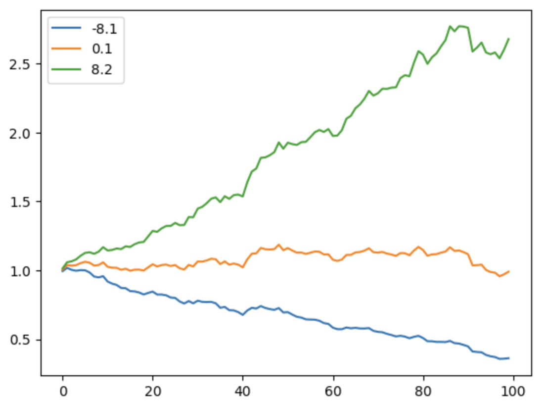
**When do we need to generate price series?** Besides the example mentioned earlier, consider this: How does the price trajectory of an asset with Sharpe ratio $S$ look? What is the relationship between price trajectory and Sharpe ratio? To answer this, we must use Monte Carlo methods to generate simulated data, calculate their Sharpe ratios, and plot them. Typically, we generate a return array following a normal distribution, weight it (to calculate Sharpe), and finally use `np.cumprod()` to calculate the price trajectory for plotting.import numpy as np
from empyrical import sharpe_ratio
import matplotlib.pyplot as plt
returns_ = np.random.normal(0, 0.02, size=100)
legend = []
for alpha in (-0.01, 0, 0.01):
returns = returns_ + alpha
prices = np.cumprod(returns + 1)
sharpe = sharpe_ratio(returns)
_ = plt.plot(prices)
legend.append(f"{sharpe:.1f}")
lines = plt.gca().lines
plt.legend(lines, legend)
From the plotted graph, we can see that when alpha is 1%, the Sharpe ratio can reach 8.2. Top domestic fund managers can achieve a Sharpe ratio of 2–3 within a year. Readers are encouraged to adjust the alpha parameter to observe the relationship between alpha and the Sharpe ratio.
2.1. The Legacy: np.random Module
Most tutorials on numpy.random found online use functions from the np.random module. Besides normal, the random package includes the following functions:
| Function | Description |
|---|---|
randint(a, b, shape) |
Generates a random integer array of shape shape within the interval (a, b). |
rand(shape) |
Generates a random array of shape shape, filled using a uniform distribution over [0, 1). |
random(shape) |
Generates a random array of shape shape, filled using a uniform distribution. |
randn(d1, d2, ...) |
Generates a random array of shape shape, filled using a normal distribution. |
standard_normal(shape) |
Generates a random array of shape shape, filled using a standard normal distribution. |
normal(loc, scale, shape) |
Generates a random array of shape shape, filled using a normal distribution, where loc is the mean and scale is the standard deviation. |
choice(a, size, replace, p) |
Randomly samples size elements from a. If replace=True, sampling with replacement is allowed; otherwise, it is not. p represents probabilities; if p=None, each element is sampled with equal probability. |
shuffle(a) |
Randomly shuffles elements in a. |
seed(seed) |
Sets the random number seed. If seed=None, the system time is used as the seed. |
It is evident that NumPy often provides multiple methods for the same functionality. To memorize these, first look at the distribution of the generated random numbers. The most basic distributions often have the simplest names: rand, randint, and random generate uniform distributions, while normal, standard_normal, and randn generate normal distributions.
Besides uniform distributions, NumPy provides generation functions for many famous distributions, such as F-distribution, Gamma distribution, Hypergeometric distribution, Beta, Weibull, etc.
Why does NumPy provide multiple functions within the same category? Some are provided for convenience to those who have used other well-known libraries (e.g., MATLAB). randn is an example; it is a function in MATLAB for generating normal random distributions, now ported to NumPy. rand is another example. random, on the other hand, is defined by NumPy according to its own API style.
The choice method has specific applications in quantitative finance. For example, we might want to randomly sample 10 stocks from a large universe for a small trial, and then consider sampling more stocks based on the results.
The seed function sets the seed for the random number generator. It is very useful for unit testing or demonstrations (both cases require generating the same sequence of random numbers consistently).
2.2. New Style: default_rng
In the previous section, we introduced some random number generation functions but did not explain their principles. NumPy generates pseudo-random numbers using a Random Number Generator (RNG). The output of an RNG is random, but identical inputs always produce identical outputs. Every method we call is essentially a sampling action on this sequence (based on the input size/shape).
In the numpy.random module, there exists a global RNG. When we call specific random functions, we are actually generating random numbers through this global RNG. This global RNG is always initialized by someone calling the seed method on it. This can cause issues because you may not know when, where, or with which parameter the seed was reset by someone else.
For this reason, it is no longer recommended to directly use these methods from the numpy.random module. A better approach is to create an independent RNG for each specific application and call the corresponding methods on this object:
rng = np.random.default_rng(seed=123)
rng.random(size=10)rng is a RandomGenerator object. When initializing, we need to pass a seed to it. If omitted, NumPy uses the system time as the seed.
rng possesses most of the methods mentioned in the previous section, such as normal, f, gamma, etc. However, methods ported from MATLAB no longer appear on this object.
Additionally, randint is replaced by rng.integers.
Furthermore, the random number generator object produced by default_rng uses the PCG64 algorithm. Compared to the algorithm used in previous versions, it not only returns statistically better random numbers but is also 4 times faster.
warning
NumPy also contains a `RandomState` class. It uses the slower Mersenne Twister to generate pseudo-random numbers. This class is now deprecated and no longer recommended.We have introduced the functionality of choice. Now, let us provide an example of how to use choice to balance a dataset.
In supervised learning, we often encounter imbalanced data. For instance, we want to train a classifier, but the class distribution in the training set is uneven. We can use the choice method to perform under-sampling or over-sampling to resolve this issue.
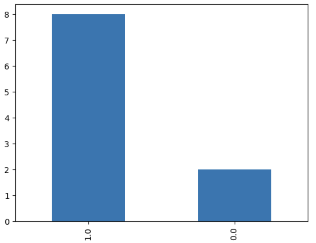
To facilitate understanding, we first generate an imbalanced training dataset. This dataset has 3 columns: the first two are features (think of them as factor features), and the third is the label.
import pandas as pd
import numpy as np
rng = np.random.default_rng(seed=42)
x = rng.random((10,3))
x[:,-1] = rng.choice([0,1], len(x), p=[0.2, 0.8])We visualize this dataset using the following method to verify that it is indeed imbalanced.
df = pd.DataFrame(x, columns=['factor1', 'factor2', 'label'])
df.label.value_counts().plot(kind='bar')The result is:
To obtain a new balanced dataset from this, we have two approaches:
- Under-sampling: Sample part of the majority class data so that its count equals that of the minority class.
- Over-sampling: Copy part of the minority class data so that its count equals that of the majority class.
The following example demonstrates under-sampling:
labels, counts = np.unique(x[:,-1], return_counts=True)
# 最小分类的标签
min_label = labels[np.argmin(counts)]
# 最小分类样本的数量,作为 UNDER SAMPLING 的样本数量
min_label_count = np.min(counts)
# 最小分类无须抽取,全部提取
results = [
x[x[:,-1] == min_label]
]
# 对其它分类标签进行遍历,需要先剔除最小分类
for label in np.delete(labels, np.argmin(counts)):
sampled = rng.choice(x[x[:,-1]== label], min_label_count)
results.append(sampled)
np.concatenate(results)This code first finds the minority class and its count, then iterates through each label, using rng.choice to randomly sample the minority class count from other classes, and finally concatenates all subsets.
This example code can be applied to scenarios with multiple labels. To perform over-sampling, simply replace min with max.
3. IO Operations
We rarely use NumPy directly to read and write files. Improving IO read/write performance has never been NumPy’s focus, so a brief understanding is sufficient.
3.1. Reading and Writing CSV Files
NumPy can read data from CSV-formatted text files, primarily using the following methods:
| API | Description |
|---|---|
loadtxt |
Parses tabular data in text format. |
savetxt |
Saves data as a text file. |
genfromtxt |
Same as above, but allows missing values in data, offering more advanced usage. |
recfromtxt |
A shortcut for genfromtxt, automatically inferring a record array. |
recfromcsv |
Same as above; if the delimiter is a comma, no additional specification is needed. |
We briefly demonstrate the usage of each with the following examples:
import io
import numpy
buffer = io.StringIO("""1,2""")
# 默认情况下,LOADTXT 只能读取浮点数
numpy.loadtxt(buffer, delimiter=",")This outputs the array array([1., 2.]).
buffer = io.StringIO("""1,2,hello""")
# 通过指定 DTYPE 参数,可以读取其它类型
numpy.loadtxt(buffer, delimiter=",", dtype=[("age", "i4"), ("score", "f4"), ("name", "U8")])This yields a Structured Array, where the third column is of string type. If we do not specify the dtype parameter, loadtxt will fail to parse.
buffer = io.StringIO("""
1,2,hello
""")
numpy.genfromtxt(buffer, delimiter=",")Here, we used genfromtxt to load data without specifying the dtype parameter. genfromtxt parses non-numeric columns as nan. Therefore, this code outputs: array([1., 2., nan]).
Now, we add the dtype parameter to genfromtxt:
buffer = io.StringIO("""
1,2,hello
""")
numpy.genfromtxt(buffer, delimiter=",", dtype=[("age", "i4"), ("score", "f4"), ("name", "U8")])The result we obtain is: array((1, 2., 'hello'), dtype=[('age', '<i4'), ('score', '<f4'), ('name', '<U8')]). Note that it is a Structured Array.
recfromtxt does not require dtype; it automatically infers data types.
buffer = io.StringIO("""
1,2,hello
""")
numpy.recfromtxt(buffer,delimiter=",")This code outputs rec.array((1, 2, b'hello'), dtype=[('f0', '<i8'), ('f1', '<i8'), ('f2', 'S5')]). If the inference is inaccurate, we can manually add the dtype parameter.
If we use recfromcsv, we can even omit the delimiter parameter.
buffer = io.StringIO("""
age,score,name
1,2,hello
""")
numpy.recfromcsv(buffer)The output is the same as the previous example.
For speed considerations, we can also use other libraries to parse CSV files and then convert them into NumPy arrays. For example:
# 利用 CSV.READER() 来解析,比 NUMPY 快 8 倍
np.asarray(list(csv.reader()))
# 利用 PANDAS 来解析,比 NUMPY 快 22 倍
pd.read_csv(buffer).to_records()3.2. Reading and Writing Binary Files
If we do not need to exchange data with external systems and the data is self-produced and self-consumed, we can also use binary files to save data.
Use the numpy.save function to save a single array as a binary file, and use the numpy.load function to read data saved by numpy.save. Files saved this way have the .npy extension.
To save multiple arrays, use the savez command. Files saved this way have the .npz extension.
For more complex requirements, libraries such as Hdf5 or pyarrow can be used to save data.
Mastering Numpy for Quant Finance: Time, Strings, and Vectorization
4. Dates and Times
Some third-party data sources deliver market data as strings or integers (Unix epoch time). For instance, many akshare and tushare APIs return string-formatted data, while QMT often represents timestamps as integers. Mastering the conversion between these formats, Numpy’s datetime objects, and Python’s native datetime objects is essential.
However, handling dates and times is notoriously complex in any programming language.
info
Few programmers or researchers realize this: dates and times are not objective mathematical or physical concepts. Time zones, daylight saving time (DST), and leap seconds are political and legal constructs. Some regions have adopted and later abolished DST. Leap second decisions are made ad hoc by a committee annually.These factors mean we cannot rely on a simple mathematical formula to calculate time, especially when converting between time zones.
An object without a time zone is timezone-naive; otherwise, it is timezone-aware. This distinction applies only to time objects (e.g., datetime.datetime in Python), not date objects (e.g., datetime.date).
import pytz
import datetime
# 通过 DATETIME.NOW() 获得的时间没有时区信息
# 返回的是标准时间,即 UTC 时间,等同于调用 UTCNOW()
now = datetime.datetime.now()
print(f"now() without param: {now}, 时区信息{now.tzinfo}")
now = datetime.datetime.utcnow()
print(f"utcnow: {now}, 时区信息{now.tzinfo}")
# 构造 TIMEZONE 对象
cn_tz = pytz.timezone('Asia/Shanghai')
now = datetime.datetime.now(cn_tz)
print(f"现在时间{now}, 时区信息{now.tzinfo}")print("现在日期:", now.date())
try:
print(now.date().tzinfo)
except AttributeError:
print("日期对象没有时区信息")The code above outputs:
now() 不带参数:2024-05-19 11:03:41.550328, 时区信息 None
utcnow: 2024-05-19 11:03:41.550595, 时区信息 None
现在时间 2024-05-19 19:03:41.550865+08:00, 时区信息 Asia/Shanghai
现在日期:2024-05-19
日期对象没有时区信息Given space constraints, we will only briefly touch upon time issues. Our primary focus here is how Numpy represents dates/times, how to compare and convert them, and how to interact with Python objects.
In Numpy, dates/times are always represented as 64-bit integers (np.datetime64), associated with a metadata structure indicating the unit (e.g., nanoseconds, seconds). np.datetime64 has no concept of time zones.
tm = np.datetime64('1970-01-01T00:00:00')
print(tm)
print(tm.dtype)This displays as:
1970-01-01T00:00:00
datetime64[s]Here, [s] denotes the time unit. Other common units include [ms], [us], and [ns].
Besides parsing from strings, we can directly convert Python objects to np.datetime64 and vice versa:
tm = np.datetimet64(datetime.datetime.now())
print(tm)
print(tm.item())
print(tm.astype(datetime.datetime))Next, let’s look at batch conversion between different formats, which is common when handling market data from third-party sources like akshare, tushare, or QMT.
First, we construct a time array. Note that we will use np.timedelta64 for time differences:
now = np.datetime64(datetime.datetime.now())
arr = np.array([now + np.timedelta64(i, 'm') for i in range(3)])
arrThe output is:
array(['2024-05-19T12:57:47.349178',
'2024-05-19T12:58:47.349178',
'2024-05-19T12:59:47.349178'],
dtype='datetime64[us]')We can convert the time array to Python time objects using np.datetime64.astype():
time_arr = arr.astype(datetime.datetime)
# 转换后的数组,每个元素都是 TIMEZONE NAIVE 的 DATETIME 对象
print(type(time_arr[0]))
# !!! 技巧
# 如何把 NP.DATETIME64 数组转换为 PYTHON DATETIME.DATE 数组?
date_arr = arr.astype('datetime64[D]').astype(datetime.date)
# 或者 -- 两者的容器不一样
date_arr = arr.astype('datetime64[D]').tolist()
print(type(date_arr[0]))The key point is that the arr array we generated earlier has elements of type np.datetime64[us]. Converting it to Python datetime.date would lose precision, so Numpy requires us to explicitly specify the conversion type.
How do we convert a string-represented time array to a Numpy datetime64 object array? The answer is still the astype() method.
# 将时间数组转换为字符串数组
str_arr_time = arr_time.astype(str)
print(str_arr_time)
# 再将字符串数组转换为 DATETIME64 数组,精度指定为 D
str_arr_time.astype('datetime64[D]')The result is:
array(['2024-05-19T12:57:47.349178',
'2024-05-19T12:58:47.349178',
'2024-05-19T12:59:47.349178'],
dtype='datetime64[us]')
array([
'2024-05-19',
'2024-05-19'],
dtype='datetime64[D]')Finally, here is an example of converting the trading calendar format obtained from QMT. In QMT, we use get_trading_dates to retrieve the trading calendar, which returns an integer array where each element is the number of milliseconds since the Unix epoch.
We can convert it using the following method:
import numpy as np
days = get_trading_dates('SH', start_time='', end_time='', count=10)
np.array(days, dtype='datetime64[ms]').astype(datetime.date)QMT does not provide a direct solution for trading calendar conversion but offers a way to convert Unix epoch timestamps to Python time objects (still represented as strings):
import time
def conv_time(ct):
'''
conv_time(1476374400000) --> '20161014000000.000'
'''
local_time = time.localtime(ct / 1000)
data_head = time.strftime('%Y%m%d%H%M%S', local_time)
data_secs = (ct - int(ct)) * 1000
time_stamp = '%s.%03d' % (data_head, data_secs)
return time_stamp
conv_time(1693152000000)We need to apply this parsing method to each array element. The official solution’s advantage is that it does not depend on any third-party libraries. However, since no quantitative program works without Numpy, our solution does not add any new third-party dependencies.
String Operations
Your data source or local storage scheme likely returns security lists using Numpy Structured Arrays or Rec Arrays. Clearly, security lists must include strings, as they contain security codes and names. Some may also return regional attributes and other properties, which are often strings.
For security lists, we often perform the following queries:
- Filter stocks by board: Stocks listed on the Beijing Stock Exchange, STAR Market, and ChiNext have different trading rules from the main board. Strategies may need to be built separately for these boards, requiring filtering of the security list by board. We may also need to exclude ST stocks or newly listed IPOs. All these can be achieved through string operations.
- Market speculation analysis: Sometimes, the market engages in speculative naming trends, such as "Dragon" stocks in the Year of the Dragon, or stocks with "Dongfang" (East) or "Zhong" (China) in their names. While quantitative traders should generally avoid such speculation, we must possess the ability to analyze and understand the market.
Most string operations in Numpy are encapsulated in the numpy.char package. It provides formatting operations (e.g., left/right padding, case conversion) and search/replace operations.
The following code demonstrates how to filter ChiNext stocks from a security list:
import numpy as np
import numpy.char as nc
# 生成 STRUCTURED ARRAY, 字段有 SYMBOL, NAME, IPO DATE
arr = np.array([('600000.SH', '中国平安', '1997-08-19'),
('000001.SZ', '平安银行', '1997-08-19'),
('301301.SZ', '川宁生物', '2012-01-01')
], dtype=[('symbol', 'S10'), ('name', 'S10'), ('ipo_date', 'datetime64[D]')])
def get_cyb(arr):
mask = np.char.startswith(arr["symbol"], b"30")
return arr[mask]question
When searching for ChiNext stocks, we use `b"30"` for matching. Why use `b"30"` instead of `"30"`?Note line 11: we use startswith via np.char.startswith(). No standard numpy array object has this method.
".SZ" is the exchange code assigned by our data source to stocks. Different data sources may use different exchange codes. For example, JoinQuant data sources use .XSHG for the Shanghai Stock Exchange and .XSHE for the Shenzhen Stock Exchange. How should we convert the above code to JoinQuant’s format?
# 生成 STRUCTURED ARRAY, 字段有 SYMBOL, NAME, IPO DATE
arr = np.array([('600000.SH', '中国平安', '1997-08-19'),
('000001.SZ', '平安银行', '1997-08-19'),
('301301.SZ', '川宁生物', '2012-01-01')
], dtype=[('symbol', 'U10'), ('name', 'U10'), ('ipo_date', 'datetime64[D]')])
def translate_exchange_code(arr):
symbols = np.char.replace(arr["symbol"], ".SH", ".XSHG")
print(symbols)
symbols = np.char.replace(symbols, ".SZ", ".XSHE")
arr["symbol"] = symbols
return arr
translate_exchange_code(arr)This time, we changed the definition of symbol and name to Unicode type to avoid entering literals like b"30" during searches.
However, the output may be surprising, as we get:
array([('600000.XSH', '中国平安', '1997-08-19'),
('000001.XSH', '平安银行', '1997-08-19'),
('301301.XSH', '川宁生物', '2012-01-01')],
dtype=[('symbol', '<U10'), ('name', '<U10'), ('ipo_date', '<M8[D]')])
question
What happened? We obtained a series of symbols ending in ".XSH", which should have been strings like "600000.XSHG". Where is the error, and how should we fix it?In the above example, if we change the replacement string to an empty string, we achieve a deletion operation. We will not demonstrate this here.
The char module also provides a string equality comparison function equal:
arr = array([('301301.SZ', '川宁生物', '2012-01-01')],
dtype=[('symbol', '<U10'), ('name', '<U10'), ('ipo_date', '<M8[D]')])
arr[np.char.equal(arr["symbol"], "301301.SZ")]In this specific scenario, we can also directly use the following syntax:
arr[arr["symbol"] == "301301.SZ"]tip
There are many functions under `np.char`. How to remember them? Most of these functions are methods from Python’s `str`. If you are familiar with Pandas, you will find similar usage there. Therefore, `str` functions like `upper`, `lower`, and `strip` can be used directly.question
Starting May 10, 2024, Nanjing Chemical Fiber experienced seven consecutive limit-ups, doubling its stock price in just seven days. Are there other stocks with "Chemical Fiber" in their names? Do their price movements exhibit correlation or cross-period correlation?You may often see Numpy masked arrays used in lower-level libraries. Masked Arrays are a crucial concept in Numpy. Consider a scenario where you have a dataset containing missing data or invalid values. These "unqualified" data points might be represented as np.nan, np.inf, None, or other syntactically valid but semantically invalid values (e.g., negative case counts in a COVID-19 dataset).
How can we perform calculations on the data while maintaining the integrity of the dataset?
note
Here is a real example. You can find a COVID-19 dataset on [Kaggle](https://www.kaggle.com/datasets/atilamadai/covid19) collected and provided by Johns Hopkins University, which includes cases with negative cumulative counts.x = np.array([1, 2, 3, np.inf, np.nan, None])
np.mean(x)
np.nanmean(x)As long as the data contains np.nan, np.inf, or None, Numpy functions cannot process them. Even if the data is syntactically valid but semantically invalid, forcing Numpy to calculate yields incorrect results.
Here is a real scenario in quantitative finance: a company has zero annual profit for a year, making its Year-over-Year (YoY) profit growth incalculable the following year. If we need to use YoY data for further calculations, we must mask this year’s invalid value. Otherwise, we cannot even calculate the mean of YoY profits.
A workaround is to copy the original data and replace invalid values with np.nan. Most subsequent calculations can then use np.nan* functions. We have introduced this method before. However, if you are the data collector, you should publish the data as-is; any modification is inappropriate. If you are the data user, you should preprocess the data before calculation. But you may lack the necessary information to preprocess the data—how could you anticipate that innocuous-looking values like -1 or 0 are hidden errors?
To solve this, Numpy provides Masked Arrays. However, we will not dwell on them. Regarding Masked Arrays, we can borrow this saying: Many people do not need to know about Masked Arrays, and those who know them are already experts.
One important note: use Masked Arrays only when necessary. Contrary to intuition, Masked Arrays do not improve performance; they significantly degrade it:
import numpy as np
# NUMPY VERSION 1.24.4
g = np.random.random((5000,5000))
indx = np.random.randint(0,4999,(500,2))
g_nan = g.copy()
g_nan[indx] = np.nan
mask = np.full((5000,5000),False,dtype=bool)
mask[indx] = True
g_mask = np.ma.array(g,mask=mask)
%timeit (g_mask + g_mask)**2
# 901 MS ± 52.3 MS PER LOOP ...
%timeit (g_nan + g_nan)**2
# 109 MS ± 72.2 ΜS PER LOOP ...As shown, Masked Arrays are nearly 9 times slower.
tip
If you must perform calculations on arrays containing `np.nan`, try using the `nan*` functions in the `bottleneck` library. Since there is no `nansquare` function, but variance calculation necessarily involves squaring, we can evaluate the performance difference between Numpy and Bottleneck using `nanvar`. %timeit np.var(g_mask)
# 587 MS ± 37.9 MS PER LOOP ...
%timeit np.nanvar(g_nan)
# 281 MS ± 1.46 MS PER ...
%timeit nanvar(g_nan)
# 61 MS ± 362 ΜS PER LOOP ...Bottleneck is nearly 5 times faster than Numpy. If you use an older version of Numpy, Bottleneck will be even faster.ufuncs
ufuncs (universal functions) are an important concept in Numpy. They perform element-wise operations on two input arrays simultaneously (e.g., addition, comparison). Numpy defines approximately 61 ufuncs. These operations are implemented in low-level C and support vectorization, making them generally faster.
For example, in Numpy, there are two similar functions to find the maximum value in an array: np.max and np.maximum. The latter is a ufunc, while the former is not. Apart from usage differences, the latter is faster.
arr = np.random.normal(size=(1_000_000,))
%timeit np.max(arr)
# 801 MS ± 54.7 MS PER LOOP ...
%timeit np.maximum.reduce(arr)
# 775 MS ± 12.1 MS PER LOOP ...np.maximum, as a ufunc, is designed to accept two arguments and cannot be used directly to find the maximum value of a 1D array. In such cases, we must use the reduce operation to achieve the desired result.
Here, np.maximum is a ufunc, and reduce is one of the attributes of the ufunc object (in Python, everything is an object, including functions). Other attributes of ufunc include accumulate, outer, and reduceat.
accumulate is another commonly used attribute in ufuncs, which you may have encountered before. For example, it is used when calculating maximum drawdown:
# 模拟一个股价序列
n = 1000
xs = np.random.randn(n).cumsum()
# 最大回撤结束期
i = np.argmax(np.maximum.accumulate(xs) - xs)
# 最大回撤开始期
j = np.argmax(xs[:i])
# 最大回撤
mdd = (xs[j] - xs[i])/xs[j]
plt.plot(xs)
plt.plot([i, j], [xs[i], xs[j]], 'o', color='Red', markersize=10)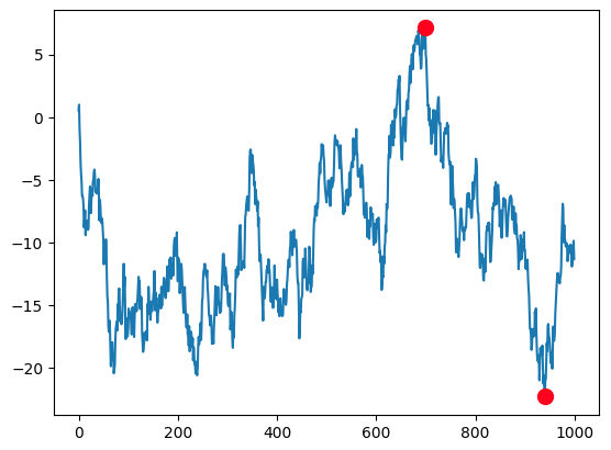
Simplicity is beauty. After using accumulate, we find that calculating maximum drawdown is as simple as two or three lines of code.
You might ask, given how useful ufuncs are, why don’t we use them more often? In fact, you likely use ufuncs every day. Many binary mathematical operations are wrappers around ufuncs.
For example, when we call A + B, we are actually calling the np.add(A, B) ufunc. They are equivalent in function and performance. Other ufuncs include logical and comparison operations. If an operation accepts two arrays as arguments, Numpy has likely implemented the corresponding ufunc. Additionally, some trigonometric functions, although accepting only one array argument, are also ufuncs.
Therefore, the ufunc functions we need to pay special attention to and learn are mainly maximum, minimum, etc. Here is another common example in quantitative scenarios using maximum—calculating the length of upper shadows.
tip
**Long upper shadows** are traces left after an asset fails to attack upward. They are helpful for analyzing subsequent stock price movements. First, capital attacked at this point, revealing its intent. Second, the attack failed, often leading to washouts (or collapse) next. Long upper shadows at the bottom of the stock price are also called "Immortals Pointing the Way" by experienced traders, indicating a higher probability of subsequent rallies. Upper shadows appearing at high levels are likely top signals. At this point, on lower-level K-lines, obvious top signals such as moving average turns may already have appeared.$$ upper_shadow = high - max(open, close) $$
The figure below shows the upper shadow:
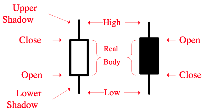
If $$upper_shadow > threshold$$, a long upper shadow is considered to have occurred (of course, upper_shadow needs to be normalized). Detecting a single day’s upper shadow is simple. The following code demonstrates how to solve this vectorially:
import numpy as np
import pandas as pd
rng = np.random.default_rng(seed=78)
matrix = rng.uniform(0.98, 1.02, (4, 30)).cumprod(axis=1)
opn = matrix[0]
close = matrix[-1]
high = np.max(matrix, axis=0)
upper_shadow = (high - np.maximum(opn, close))/close
np.round(upper_shadow, 2)Line 10’s code consists entirely of ufuncs. Here we use np.sub (subtraction), np.maximum, and np.divide (division). maximum compares elements from two equally long arrays, opn and close, element-wise, and takes the larger one to form a new array, which is also as long as opn and close.
To calculate the lower shadow length, use minimum.
"Factor Investing and Machine Learning Strategies" Course is Now Open!

Clear Goals, Strong Sense of Achievement

Why You Should Choose QuanTide’s Courses?