Low-Volatility Factor Rises in Importance After New Rules

Robert (Bob) Haugen, father of the low-volatility factor. Image via MarketWatch

In a previous post we introduced the low-turnover factor. The logic behind it is to buy where no one is looking, wait patiently for your time, and finally sell when the crowd rushes in. It is a game of positioning.

The low-volatility factor we introduce today makes a similar case for neglected stocks. Because of its low-volatility nature, it is shunned by short-term money in practice; academically, it contradicts popular theories like CAPM and EMH. When first proposed, it was therefore treated as a heresy by both Wall Street and academia. It was not until 2008 that MSCI moved into this factor with its MSCI Global Minimum Volatility Index.

Extensive empirical research shows that over decades of market history, the low-volatility factor has delivered a clear edge: the road less traveled sometimes offers the better journey.

After China's New Nine Guidelines, dividend stocks will matter much more for investors, and the low-volatility factor is excellent at identifying dividend payers and blue-chip compounders. That is the timely backdrop for this piece.

How the Low-Volatility Factor Has Performed

Since CAPM was published, Wall Street and academia have firmly believed risk and return go hand in hand: markets are efficient, and to earn higher returns investors must take more risk.

Yet Robert Haugen and his teacher, Professor James Heins, found in the 1960s-70s that, contrary to popular theory, lower-risk stocks actually delivered higher returns.

Haugen argued that the standard textbooks on investing and corporate finance were "completely wrong and need to be rewritten." His strong advocacy earned him the informal title of "father of low-volatility investing." According to research by Dr. Tim Edwards of S&P Global and co-authors, low-volatility indices beat their parent indices on a risk-adjusted basis in many countries — in Japan by almost 2x. We will skip that chart and show a cumulative return comparison instead.

Source: S&P Dow Jones Indices, 1990-2018

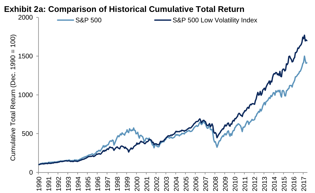
This chart compares the historical cumulative return of a low-volatility stock pool against the market (the S&P 500). In almost any period, the low-volatility factor outperformed the market in total return — not just risk-adjusted return.

Their construction: pick the 20% least volatile stocks from the S&P 500, weight them inversely to volatility, and rebalance quarterly.

The research report is educational and available as a free download at blog.quantide.cn.

In a post last Q3, MSCI disclosed the performance of its low-volatility index:

Source: MSCI

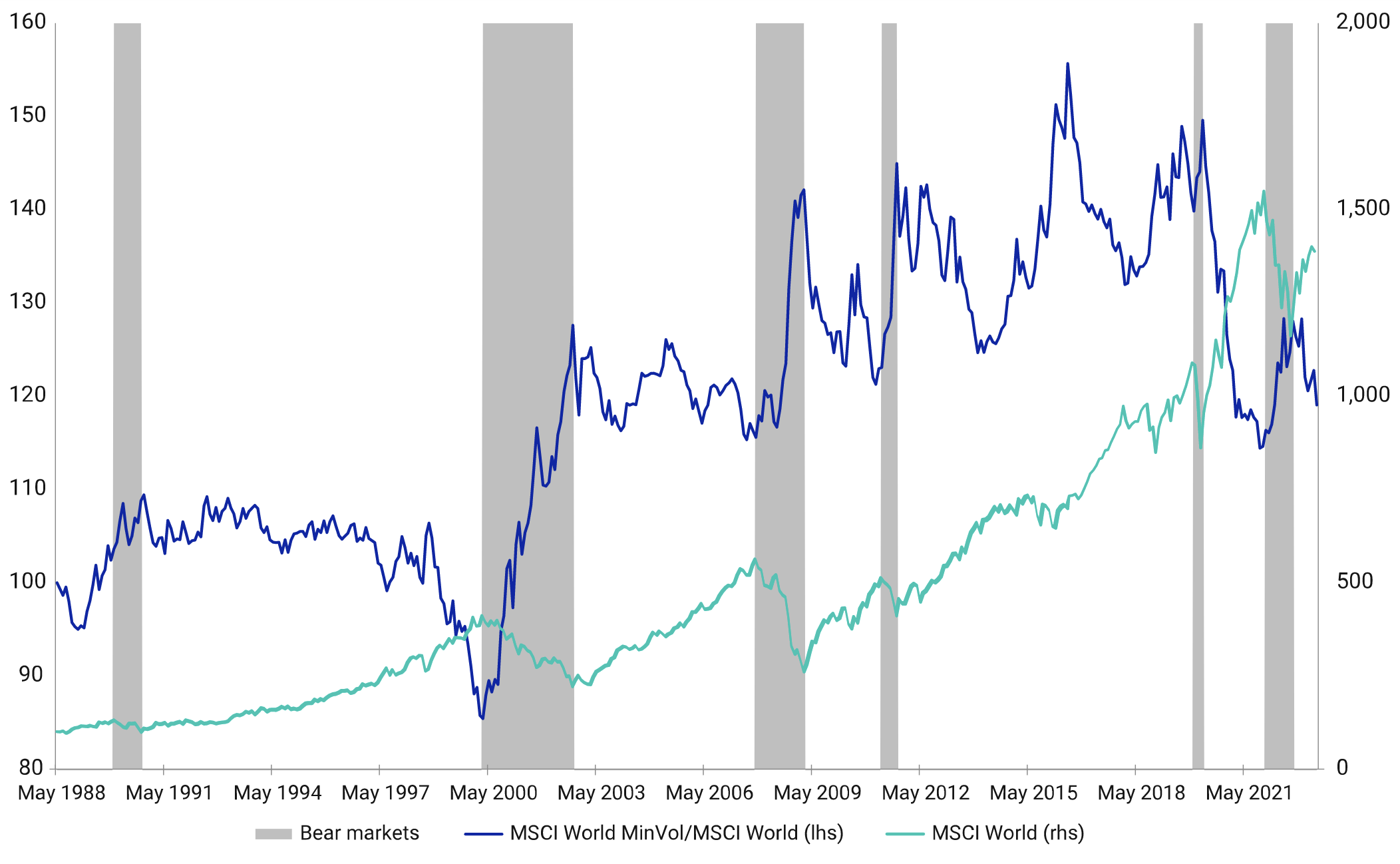
As shown above, the low-volatility factor can even rise against the market during downturns, and beats the index in most other periods as well.

Why the Low-Volatility Factor Works

Academics have used plenty of math and data to explain why low volatility works. But back to first principles: what creates low volatility? A shareholder base that believes in the company for the long term, holds mainly for dividends, and rarely trades.

Why would investors hold a stock for so long? Because the business is simple to understand (so investors do not flip-flop), the moat is deep (the competitive landscape rarely changes), and profitability is strong (at the core, it must make money). These are the companies the world cannot change (from a recent roadshow by Dan Bin).

That sounds a lot like value investing. Indeed, extensive academic work finds a strong link between the low-volatility factor and the value factor: low-volatility stocks also tend to be low price-to-book stocks. That is why blue chips and long-term dividend stocks are often low-volatility names.

There is an interesting link between the Sharpe ratio and volatility. The Sharpe ratio is a risk-adjusted return whose denominator — the standard deviation of asset returns — is a linear function of volatility.

Its creator was William Sharpe, the founder of CAPM theory. Yet supporters of low-volatility investing use low volatility as a weapon to rebel against modern finance theory represented by CAPM. In other words, when Sharpe published CAPM, he also created its own gravedigger. Very dialectical.

How to Calculate Volatility

According to Investopedia, the formula for volatility is:

$$ vol = \sqrt{var(R)}/T $$

Here T is the number of periods over which return R is measured. Some versions do not divide by T.

In finance, volatility is usually presented and compared on an annualized basis. This can be calculated with pandas:

12345bars = ...
close = bars["close"]

close.pct_change().rolling(window_size)
     .std() * (252**0.5)

For single-factor testing, we need daily volatility for each name, which is why we need the rolling version here.

Or, more simply, use the open-source empyrical library:

1234from empyrical import annual_volatility

daily_returns = close.pct_change()
annual_volatility

A Low-Volatility Strategy

In general, we do not need to test the low-volatility factor ourselves — we can use it directly for stock selection.

Note that if you screen on short-term volatility, you are very likely to pick up stocks in a downtrend. The chart below shows how the same volatility can hide completely different price paths:

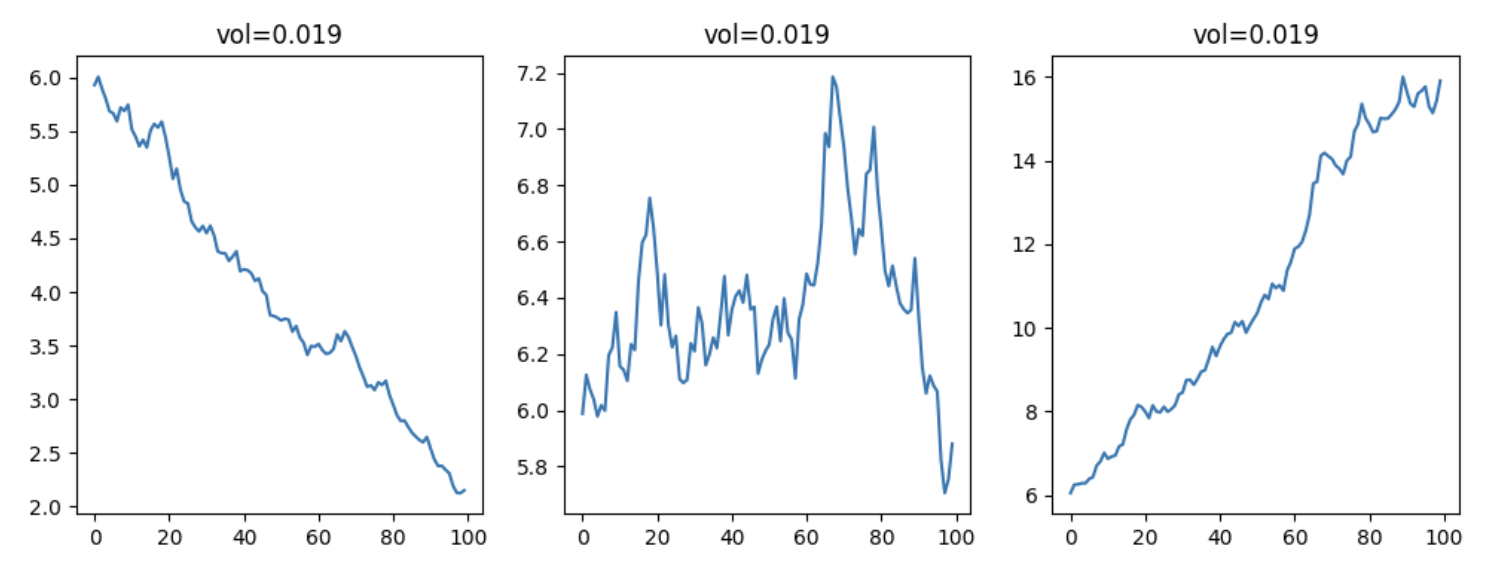
Under low-volatility conditions, judging the trend is easy: regress price, and if the fitted line slopes upward (slope > 0), the trend is up.

The key here is to first use monthly bars, at least 24 periods. Over shorter horizons, low volatility has no economic rationale behind it. The core code is:

1234567891011121314151617for symbol, name, _ in get_secs():
    bars = get_bars(symbol, 24, ...)
    if len(bars) < 24:
        continue

    close = bars["close"][-24:]
    returns = close[1:]/close[:-1] - 1
    # 计算波动率
    vol = np.std(returns)

    # 计算斜率
    a, b = np.polyfit(np.arange(24), close/close[0], degree=1)
    result.append((name, symbol, vol, a))

df = pd.DataFrame(result, columns=["name", "symbol", "vol", "slope"])

df[df.slope>0].nsmallest(10, "vol")

This gives us 10 stocks with an upward trend and the lowest volatility. When slope is close to 0, the trend cannot really be called up, so we can filter by quantile:

123quant_25 = df[df.slope>0].slope.quantile(0.25)

df[df.slope > quant_25].nsmallest(10, "vol")

Conclusion

The road less traveled sometimes offers the better journey. After the New Nine Guidelines, dividend stocks will matter much more for investors, and the low-volatility factor is excellent at identifying dividend and blue-chip stocks. If accounting data in a market is unreliable, we should use the low-volatility factor instead of the value factor. Price and volume never lie. If a once-good company recently ran into trouble, those who read financial statements are always the last to know. But the stock price reflects it in advance.