
ESG Long-Short Strategy: Does High ESG Score Mean Alpha? (With Backtest Code)
1. Introduction
Recap
Key Findings:
We construct a strategy framework for both Huazheng and Wind ESG scores: "cross-sectional layering by disclosure date, effective T+1, forward-filled to daily frequency, and equally weighted until the next disclosure." We conduct systematic backtests over the longest traceable sample period. The results are as follows:
Weak Offensive Power: High ESG scores ≠ higher returns. Throughout complete bull, bear, and volatile cycles, most periods fail to generate excess returns.
Strong Defensive Power: The advantage lies in significantly reducing volatility and drawdown, acting as a "risk shock absorber."
Market-Dependent Effectiveness: Effectiveness heavily depends on the market environment, showing prominence only in specific windows like 2019–2021.
Data Sources: Huazheng ESG (Comprehensive/E/S/G sub-scores), Wind ESG (Comprehensive). Backtests conducted separately for each provider.
Sample Frequency: ESG data is quarterly; market data is daily.
Effective Periods:
- Wind ESG: 2018–2023
- Huazheng ESG: 2008–2023
- Daily Market Data Coverage: 2008–2023
Outlier Clipping & Cleaning: Daily returns are winsorized at the default 0.5%/99.5% percentiles, excluding abnormal cases and ST (Special Treatment) stocks.
Since both Wind and Huazheng ESG data are in score format, we can easily layer the scores. After unifying the data format, we can directly call functions to perform identical layering processing on scores from different sources.
tip
Using the Quantide Research platform, the following code enables pre-downloading data:
import pandas as pd
import os
start = datetime.date(2009, 1, 1)
end = datetime.date(2023, 12, 29)
universe = -1
# Fetch all stocks
df = load_bars(start, end, -1)
df.to_parquet('daily_data.parquet')The downloaded data format is as follows:
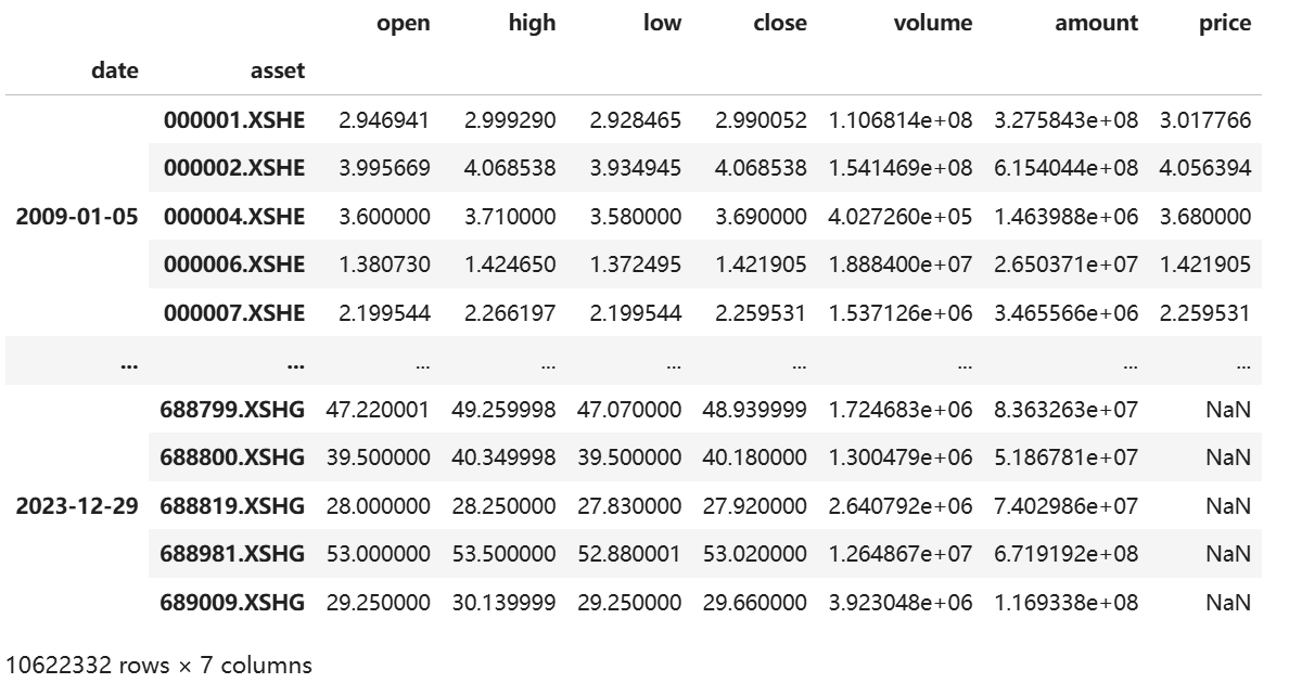
From the returned results, we can see that the research platform’s data is comprehensive, recording metrics such as trading volume and amount for each stock. This same data can be used for other daily strategy backtests.
attention
With the research data ready, we proceed to implement the ESG layering return analysis.
2. Analysis Steps
attention
First, we import the necessary libraries for analysis.
import pandas as pd
import numpy as np
import matplotlib.pyplot as plt
import quantstats as qs
import os
from datetime import datetime
import warnings
qs.extend_pandas()
warnings.filterwarnings('ignore')
plt.rcParams['font.family'] = 'WenQuanYi Zen Hei'
import matplotlib as mpl
plt.rcParams['font.sans-serif'].insert(0, 'DejaVu Sans') # 优先使用DejaVu Sans
# 创建图表输出目录
if not os.path.exists(str(get_jupyter_root_dir() / "reports/ESG/")):
os.makedirs(str(get_jupyter_root_dir() / "reports/ESG/"))
report_dir = str(get_jupyter_root_dir() / "reports/ESG/")2.1 Data Cleaning
- Read Huazheng and Wind ESG data along with full-market daily data.
- Exclude ST stocks, abnormal dates, and missing values, retaining necessary fields (stock code, date, score). Sort by date and stock code.
def preprocess_esg_data(esg_data, score_column, exclude_st=True):
"""预处理ESG数据,统一列名和格式,可选剔除ST股票"""
df = esg_data.copy()
# 统一重命名:使用列索引重命名(两个数据源格式已统一)
df = df.rename(columns={
df.columns[0]: 'stock_code', # 证券代码
df.columns[1]: 'stock_name', # 证券名称
df.columns[2]: 'date' # 日期(无论是"评级日期"还是"交易日期")
})
# 处理日期列,过滤无效日期
df['date'] = pd.to_datetime(df['date'], errors='coerce')
df = df.dropna(subset=['date'])
# 剔除ST股票(如果启用)
if exclude_st and 'stock_name' in df.columns:
st_mask = df['stock_name'].str.contains('ST', na=False)
st_count = st_mask.sum()
if st_count > 0:
df = df[~st_mask]
print(f"[INFO] 剔除ST股票:{st_count:,} 条记录")
# 保留必要的列
keep_cols = ['stock_code', 'date', score_column]
df = df[keep_cols]
df = df.dropna(subset=[score_column])
df = df.sort_values(['date', 'stock_code'])
print(f"[OK] 数据预处理完成,共 {len(df):,} 条记录")
print(f" 日期范围:{df['date'].min().strftime('%Y-%m-%d')} 至 {df['date'].max().strftime('%Y-%m-%d')}")
print(f" 股票数量:{df['stock_code'].nunique():,}")
return df
wind_esg_data = pd.read_parquet('wind_esg.parquet')
esg_wind = preprocess_esg_data(wind_esg_data, score_column='WindESG评级')2.2 Score Layering
- Perform cross-sectional ranking and layering of ESG scores for each disclosure date.
- The number of layers is adjustable (default: 10 layers). Layer 1 represents the bottom 10% of scores, and Layer 10 represents the top 10%.
This process is executed independently for Huazheng comprehensive scores, E/S/G sub-scores, and Wind ESG ratings.
def classify_score_per_period(esg_df, score_column, n_layers=5, data_source='wind'):
"""统一的评分分层函数(支持华政和Wind)"""
df = esg_df.copy().sort_values(['date','stock_code'])
def _cut_period(g):
# 对每个披露日期的截面数据分层(robust to ties)
try:
g['layer'] = pd.qcut(
g[score_column].rank(method='first'),
q=n_layers, labels=False, duplicates='drop'
) + 1
except Exception:
ranks = g[score_column].rank(method='first')
g['layer'] = pd.cut(ranks, bins=n_layers, labels=False, include_lowest=True) + 1
return g
df = df.groupby('date', group_keys=False).apply(_cut_period)
print(f"[OK] {data_source}评分分层完成(每个披露日截面分{n_layers}层)")
print(f"各层总体分布:")
layer_dist = df.groupby('layer').size()
for layer, count in layer_dist.items():
print(f" Layer {layer}: {count:,} ({count/len(df)*100:.1f}%)")
return df[['stock_code','date','layer']]
esg_wind_classified = classify_score_per_period(esg_wind, 'WindESG评级', n_layers=10, data_source='Wind')2.3 Daily Return Calculation
Calculate the daily return for each stock from the full-market daily data, excluding outliers and extreme price limits (default winsorization at the 0.5% percentile). This ensures a clean sample, preventing extreme volatility from distorting the mean within each layer.
daily_data = pd.read_parquet('daily_data.parquet')
def prepare_daily_returns(daily_df, price_col='close', min_price=0.01,winsor_p=0.005):
"""从日线数据中计算收益率(含清洗和去极值)"""
print("正在准备日线收益率数据...")
df = daily_df.reset_index().rename(columns={'asset': 'stock_code'})
df['date'] = pd.to_datetime(df['date'])
df = df[['stock_code','date',price_col]].copy()
# 价格数值化与过滤:非正、极小值、缺失全滚粗
df[price_col] = pd.to_numeric(df[price_col], errors='coerce')
df = df.dropna(subset=[price_col])
df = df[df[price_col] > min_price]
df = df.sort_values(['stock_code','date'])
ret = df.groupby('stock_code')[price_col].pct_change()
# 干掉 inf/-inf、超大绝对值
ret = ret.replace([np.inf, -np.inf], np.nan)
lo = ret.quantile(winsor_p)
hi = ret.quantile(1 - winsor_p)
ret = ret.clip(lo, hi)
df['return'] = ret
df = df.dropna(subset=['return'])
# 可选:把 |r|>30% 的样本数量打个日志
outlier_cnt = (df['return'].abs() > 0.3).sum()
if outlier_cnt > 0:
print(f"[WARN] |return|>30% 样本: {outlier_cnt:,}")
print(f"[OK] 日线数据处理完成,共 {len(df):,} 条记录")
print(f" 股票数量:{df['stock_code'].nunique():,}")
print(f" 平均日收益率:{df['return'].mean():.4%}")
return df[['stock_code','date','return',price_col]]
daily_returns = prepare_daily_returns(daily_data)
2.4 Extending Ratings to Daily Frequency
From quarterly to daily: A three-step approach.
- Cross-sectional Layering: Divide each disclosure day into N layers based on percentiles (10 layers in this article).
- Layer Label Holding: Carry the layer label from the disclosure date forward until the next disclosure date updates it.
- T+1 Effectiveness: To avoid look-ahead bias, the layering signal begins affecting returns on the next trading day.
Extending quarterly ESG ratings to a daily frequency with a T+1 effectiveness mechanism (i.e., the rating takes effect one trading day after disclosure) ensures that the signal and return timelines are not contaminated. Rebalancing occurs the day after the rating is published.
def expand_to_daily_with_t1(esg_layers, daily_df):
"""将季度ESG评级扩展到日线,并实施T+1延迟"""
print("正在将季度ESG数据扩展到日线(T+1延迟)...")
# 统一股票代码格式
def convert_stock_code(code):
code = str(code)
if code.endswith('.SZ'):
return code.replace('.SZ', '.XSHE')
elif code.endswith('.SH'):
return code.replace('.SH', '.XSHG')
return code
esg = esg_layers[['stock_code','date','layer']].copy()
esg['stock_code'] = esg['stock_code'].apply(convert_stock_code)
esg['date'] = pd.to_datetime(esg['date'])
dly = daily_df[['stock_code','date','return']].copy()
dly['stock_code'] = dly['stock_code'].astype(str)
dly['date'] = pd.to_datetime(dly['date'])
# 合并
merged = dly.merge(esg, on=['stock_code','date'], how='left')
merged = merged.sort_values(['stock_code','date'])
# 前向填充最新的layer
merged['layer'] = merged.groupby('stock_code')['layer'].ffill()
# T+1延迟:今天的收益使用昨天的layer
merged['layer'] = merged.groupby('stock_code')['layer'].shift(1)
merged = merged.dropna(subset=['layer'])
merged['layer'] = merged['layer'].astype(int)
print(f"[OK] 合并完成,共 {len(merged):,} 条记录(含T+1延迟)")
return merged
daily_with_wind = expand_to_daily_with_t1(esg_wind_classified, daily_returns)
# 清洗
daily_with_wind = daily_with_wind.replace([np.inf, -np.inf], np.nan)
daily_with_wind = daily_with_wind[daily_with_wind['return'].between(-0.5, 0.5)]
print(f"[INFO] 清洗后Wind数据:{len(daily_with_wind):,} 条记录")
2.5 Layered Backtest
- Calculate the equally weighted average return for each layer on each trading day, filtering out layers with insufficient constituents (default: ≥10 stocks).
- Use the QuantStats library to quickly calculate key performance indicators for each layer and the long-short portfolio: annualized return, volatility, Sharpe ratio, max drawdown, Calmar ratio, Sortino ratio, win rate, etc.
def backtest_hold_between_events(dly_with_layer, min_names_per_layer_day=10):
"""执行分层回测(使用quantstats简化指标计算)"""
print("正在执行分层回测(使用quantstats)...")
df = dly_with_layer.copy()
# 诊断:层内日样本数分布
print("层内日样本数分布:")
print(df.groupby(['layer'])['date'].nunique().describe())
print("单日层内成分数的分位:")
print(df.groupby(['date','layer'])['stock_code'].nunique().quantile([.1,.25,.5,.75,.9]))
# 先统计每天每层有多少只股票
counts = df.groupby(['date','layer'])['stock_code'].nunique()
# 仅保留成分数≥阈值的层日(避免"一只妖股带飞全层")
valid = counts[counts >= min_names_per_layer_day].index
df = df.set_index(['date','layer']).loc[valid].reset_index()
print(f"[INFO] 过滤后保留 {len(df):,} 条记录(每层日至少{min_names_per_layer_day}只股票)")
# 每日等权layer收益;空缺日留作NaN
layer_daily = df.groupby(['date','layer'])['return'].mean().unstack()
# 确保索引是DatetimeIndex
if not isinstance(layer_daily.index, pd.DatetimeIndex):
layer_daily.index = pd.to_datetime(layer_daily.index)
# 对数收益率
def _cumprod_stable(s):
r = s.dropna()
if len(r) == 0:
return pd.Series(index=s.index)
logcum = np.log1p(r).cumsum()
cr = np.exp(logcum)
return cr.reindex(s.index).ffill()
cum = layer_daily.apply(_cumprod_stable)
# ========== 使用quantstats计算各层统计指标(更简洁!)==========
stats = {}
for layer in layer_daily.columns:
r = layer_daily[layer].dropna()
if len(r) == 0:
continue
stats[f'Layer_{layer}'] = {
'Total_Return': qs.stats.comp(r),
'Annualized_Return': qs.stats.cagr(r),
'Volatility': qs.stats.volatility(r),
'Sharpe_Ratio': qs.stats.sharpe(r),
'Max_Drawdown': qs.stats.max_drawdown(r),
'Calmar_Ratio': qs.stats.calmar(r),
'Sortino_Ratio': qs.stats.sortino(r),
'Win_Rate': qs.stats.win_rate(r),
}
# 计算多空策略
long_short_returns = None
long_short_cumulative = None
if len(layer_daily.columns) >= 2:
top = layer_daily.columns.max()
bot = layer_daily.columns.min()
# 只在两层都有数据的日期计算多空
r_ls = pd.concat([layer_daily[top], layer_daily[bot]], axis=1).dropna()
ls = r_ls.iloc[:,0] - r_ls.iloc[:,1]
long_short_returns = ls
long_short_cumulative = (1 + ls).cumprod()
# 使用quantstats计算多空策略指标
stats['Long_Short'] = {
'Total_Return': qs.stats.comp(ls),
'Annualized_Return': qs.stats.cagr(ls),
'Volatility': qs.stats.volatility(ls),
'Sharpe_Ratio': qs.stats.sharpe(ls),
'Max_Drawdown': qs.stats.max_drawdown(ls),
'Calmar_Ratio': qs.stats.calmar(ls),
'Sortino_Ratio': qs.stats.sortino(ls),
'Win_Rate': qs.stats.win_rate(ls),
}
print("[OK] 回测完成!")
return {
'daily_returns': layer_daily,
'cumulative_returns': cum,
'statistics': stats,
'long_short_returns': long_short_returns,
'long_short_cumulative': long_short_cumulative
}
#计算开始
wind_results = backtest_hold_between_events(daily_with_wind, min_names_per_layer_day=10)
print("\nWind评分回测结果:")
print(pd.DataFrame(wind_results['statistics']).T.to_string())
2.6 Visualization and Report Output
Use QuanStats to generate four types of charts:
- Cumulative return curves for each layer
- Long-short strategy returns and drawdowns
- Comparison of core performance indicators
- Summary table of indicators
# 保存结果
all_results = {}
all_results['Wind评分'] = wind_results
def plot_backtest_results(results, title='ESG_Backtest', save_path=f'{report_dir}'):
"""增强的可视化回测结果(使用quantstats风格)"""
cumulative_returns = results['cumulative_returns']
statistics = results['statistics']
long_short_cumulative = results['long_short_cumulative']
long_short_returns = results['long_short_returns']
# 根据实际层数动态生成配色方案
n_layers = len(cumulative_returns.columns)
# 使用 tab20 配色方案支持更多层数,如果层数少用 Set2
if n_layers <= 8:
colors = plt.cm.Set2(np.linspace(0, 1, n_layers))
else:
colors = plt.cm.tab20(np.linspace(0, 1, n_layers))
fig, axes = plt.subplots(2, 2, figsize=(18, 12))
fig.patch.set_facecolor('white')
# 1. 各层累计收益
ax1 = axes[0,0]
for i, layer in enumerate(cumulative_returns.columns):
ax1.plot(cumulative_returns.index, cumulative_returns[layer],
label=f'Layer {layer}', linewidth=2.5, color=colors[i], alpha=0.8)
ax1.axhline(y=1, color='black', linestyle='--', alpha=0.3, linewidth=1)
ax1.set_title('Cumulative Returns by Layer', fontsize=14, fontweight='bold', pad=15)
ax1.set_xlabel('Date', fontsize=11)
ax1.set_ylabel('Cumulative Return', fontsize=11)
ax1.legend(loc='best', framealpha=0.9, fontsize=10)
ax1.grid(True, alpha=0.3, linestyle=':', linewidth=0.5)
ax1.set_facecolor('#f7f7f7')
# 2. 多空策略 + 回撤
ax2 = axes[0,1]
if long_short_cumulative is not None and long_short_returns is not None:
# 绘制累计收益
ax2.plot(long_short_cumulative.index, long_short_cumulative,
linewidth=3, color='#2E7D32', label='Long-Short', alpha=0.9)
ax2.axhline(y=1, color='black', linestyle='--', alpha=0.3, linewidth=1)
# 添加回撤阴影
drawdown = qs.stats.to_drawdown_series(long_short_returns)
ax2_twin = ax2.twinx()
ax2_twin.fill_between(drawdown.index, drawdown * 100, 0,
color='#D32F2F', alpha=0.3, label='Drawdown')
ax2_twin.set_ylabel('Drawdown (%)', fontsize=10, color='#D32F2F')
ax2_twin.tick_params(axis='y', labelcolor='#D32F2F')
ax2_twin.legend(loc='lower right', framealpha=0.9, fontsize=9)
ax2.set_title('Long-Short Strategy with Drawdown', fontsize=14, fontweight='bold', pad=15)
ax2.set_xlabel('Date', fontsize=11)
ax2.set_ylabel('Cumulative Return', fontsize=11)
ax2.legend(loc='upper left', framealpha=0.9, fontsize=10)
ax2.grid(True, alpha=0.3, linestyle=':', linewidth=0.5)
ax2.set_facecolor('#f7f7f7')
# 3. 绩效指标对比
ax3 = axes[1,0]
metrics = ['Total_Return', 'Sharpe_Ratio', 'Calmar_Ratio'] # 与标签/颜色一一对应
metric_labels = ['Ann. Return', 'Sharpe Ratio', 'Calmar Ratio']
metric_colors = ['#66C2A5', '#FC8D62', '#8DA0CB']
if not strat_keys:
ax3.axis('off') # 没有可画的就关掉子图
else:
x = np.arange(len(strat_keys))
width = 0.25
for i, (metric, label, color) in enumerate(zip(metrics, metric_labels, metric_colors)):
vals = [statistics[k].get(metric, 0) for k in strat_keys]
ax3.bar(x + i*width, vals, width, label=label,
color=color, alpha=0.8, edgecolor='white', linewidth=1.5)
ax3.set_title('Performance Metrics Comparison', fontsize=14, fontweight='bold', pad=15)
ax3.set_xlabel('Strategy', fontsize=11)
ax3.set_ylabel('Value', fontsize=11)
ax3.set_xticks(x + width)
ax3.set_xticklabels([str(k).replace('_', ' ') for k in strat_keys],
rotation=15, ha='right', fontsize=9)
ax3.legend(loc='best', framealpha=0.9, fontsize=10)
ax3.grid(True, alpha=0.3, axis='y', linestyle=':', linewidth=0.5)
ax3.set_facecolor('#f7f7f7')
# 4. 统计表格(选择关键指标)
ax4 = axes[1,1]
ax4.axis('tight')
ax4.axis('off')
key_metrics = ['Total_Return', 'Annualized_Return', 'Sharpe_Ratio',
'Max_Drawdown','Volatility', 'Win_Rate']
stats_df = pd.DataFrame(statistics).T[key_metrics].round(2)
# 表格
table = ax4.table(cellText=stats_df.values,
rowLabels=stats_df.index,
colLabels=[col.replace('_', ' ') for col in stats_df.columns],
cellLoc='center',
loc='center',
bbox=[0, 0, 1, 1])
table.auto_set_font_size(False)
table.set_fontsize(9)
table.scale(1, 2.2)
# 表头样式
for i in range(len(stats_df.columns)):
table[(0, i)].set_facecolor('#4CAF50')
table[(0, i)].set_text_props(weight='bold', color='white')
# 行标签样式
for i in range(len(stats_df)):
table[(i+1, -1)].set_facecolor('#E8F5E9')
table[(i+1, -1)].set_text_props(weight='bold')
ax4.set_title('Performance Statistics', fontsize=14, fontweight='bold', pad=15)
plt.suptitle(title.replace('_', ' '), fontsize=16, fontweight='bold', y=0.995)
plt.tight_layout()
# 保存图表
filename = f'{save_path}/{title}.png'
plt.savefig(filename, dpi=300, bbox_inches='tight', facecolor='white')
print(f"[OK] 图表已保存:{filename}")
plt.close()
return fig
# 绘图
plot_backtest_results(wind_results, title='Wind_ESG_Score')
Additionally, an HTML report from QuantStats is automatically generated for each strategy.
def generate_quantstats_report(returns, output_file, title='ESG Strategy Report'):
print(f"正在生成quantstats报告:{output_file}")
# 1) 保证是 Series,索引为 DatetimeIndex
if isinstance(returns, pd.DataFrame):
returns = returns.iloc[:, 0]
returns = returns.dropna().astype(float)
if not isinstance(returns.index, pd.DatetimeIndex):
returns.index = pd.to_datetime(returns.index)
if not returns.name:
returns.name = 'Strategy'
# 2) 构造零基准,长度与索引匹配
benchmark = pd.Series(0.0, index=returns.index, name='Zero')
# 3) 生成报告
qs.reports.html(
returns,
benchmark=benchmark,
title=title,
output=output_file
)
print(f"[OK] Quantstats报告已保存")
# 生成Wind多空策略的quantstats完整报告
if wind_results['long_short_returns'] is not None:
generate_quantstats_report(
wind_results['long_short_returns'],
output_file = f'{report_dir}/wind_longshort_report.html',
title='Wind评分多空策略报告'
)3. Wind Results Analysis
After executing the above code, we obtain the Wind ESG investment results, as shown below::
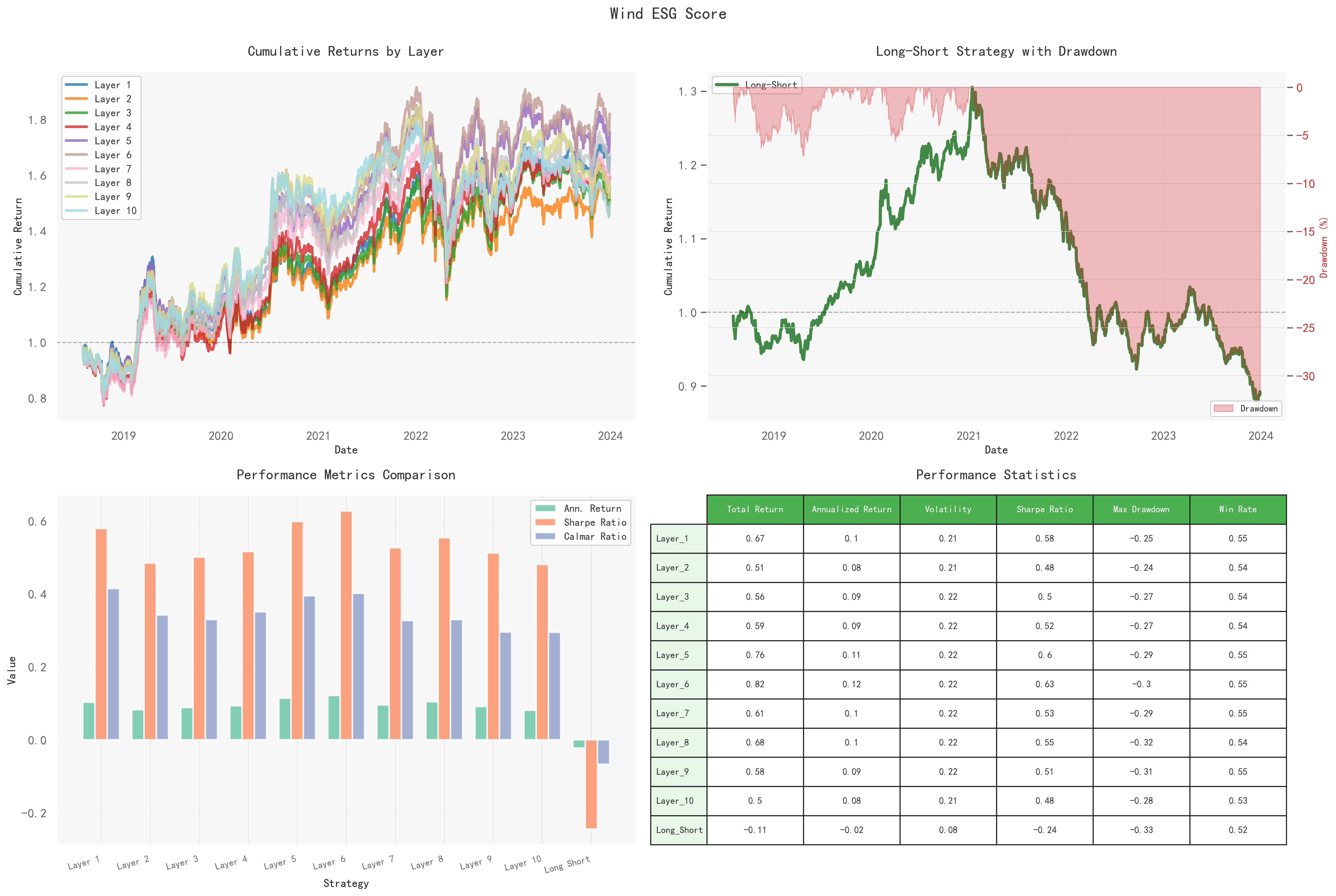 The differences between layers are limited, with frequent crossovers between layers; monotonicity does not hold.
We observe the long-short return chart:
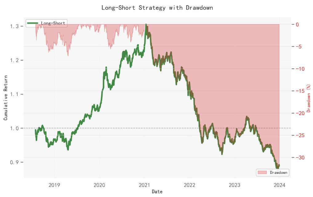
The strategy covers a relatively short period, experiencing a "2019–2021 uptrend followed by a 2022–2023 drawdown" cycle. It is effective in stages but then fades.
So, are high-ESG companies completely useless?
| Layer | Total Return | Annualized Return | Volatility | Sharpe Ratio | Max Drawdown | Win Rate |
|---|---|---|---|---|---|---|
| 1 | 0.67 | 0.1 | 0.21 | 0.58 | -0.25 | 0.55 |
| 2 | 0.51 | 0.08 | 0.21 | 0.48 | -0.24 | 0.54 |
| 3 | 0.56 | 0.09 | 0.22 | 0.5 | -0.27 | 0.54 |
| 4 | 0.59 | 0.09 | 0.22 | 0.52 | -0.27 | 0.54 |
| 5 | 0.76 | 0.11 | 0.22 | 0.6 | -0.29 | 0.55 |
| 6 | 0.82 | 0.12 | 0.22 | 0.63 | -0.3 | 0.55 |
| 7 | 0.61 | 0.1 | 0.22 | 0.53 | -0.29 | 0.55 |
| 8 | 0.68 | 0.1 | 0.22 | 0.55 | -0.32 | 0.54 |
| 9 | 0.58 | 0.09 | 0.22 | 0.51 | -0.31 | 0.55 |
| 10 | 0.5 | 0.08 | 0.21 | 0.48 | -0.28 | 0.53 |
| Long-Short | -0.11 | -0.02 | 0.08 | -0.24 | -0.33 | 0.52 |
The answer is no. According to the final backtest results, although Layer 10 (the high-ESG group) has the lowest annualized return, its max drawdown is also relatively low.
High-ESG stocks act as a safe haven. They do not generate significant returns, but they also do not suffer large losses.
4. Huazheng Data Multi-dimensional Analysis
Next, we call the functions written above to conduct layered backtest tests on Huazheng ESG total scores and individual sub-scores:
huazheng_esg_data = pd.read_parquet('hz_esg.parquet')
print("准备日线收益率数据")
daily_returns = prepare_daily_returns(daily_data)
# 华政ESG 4个分层回测
huazheng_scores = [
('综合得分', '综合得分'),
('E得分', 'E得分'),
('S得分', 'S得分'),
('G得分', 'G得分')
]
for score_name, score_col in huazheng_scores:
print(f"\n" + "="*80)
print(f"华政{score_name}回测")
print("="*80)
# 预处理数据
esg_huazheng = preprocess_esg_data(huazheng_esg_data, score_column=score_col)
# 分层(使用统一函数)
esg_huazheng_classified = classify_score_per_period(esg_huazheng, score_col,
n_layers=10, data_source=f'华政{score_name}')
# 扩展到日线
daily_with_huazheng = expand_to_daily_with_t1(esg_huazheng_classified, daily_returns)
# 清洗
daily_with_huazheng = daily_with_huazheng.replace([np.inf, -np.inf], np.nan)
daily_with_huazheng = daily_with_huazheng[daily_with_huazheng['return'].between(-0.5, 0.5)]
print(f"[INFO] 清洗后华政{score_name}数据:{len(daily_with_huazheng):,} 条记录")
# 回测
huazheng_results = backtest_hold_between_events(daily_with_huazheng, min_names_per_layer_day=10)
print(f"\n华政{score_name}回测结果:")
print(pd.DataFrame(huazheng_results['statistics']).T.to_string())
# 保存结果
all_results[f'华政{score_name}'] = huazheng_results
# 绘图
plot_backtest_results(huazheng_results, title=f'Huazheng_{score_name}')
print(f"[OK] 华政{score_name}多空策略报告已生成")
generate_quantstats_report(
huazheng_results['long_short_returns'],
output_file=f'{report_dir}/huazheng_{score_name}_longshort_report.html',
title=f'华政{score_name}多空策略报告'
)Huazheng provides more rating data, including separate E, S, and G scores. Therefore, we can draw four layered return analysis charts:
4.1 Huazheng Comprehensive Score
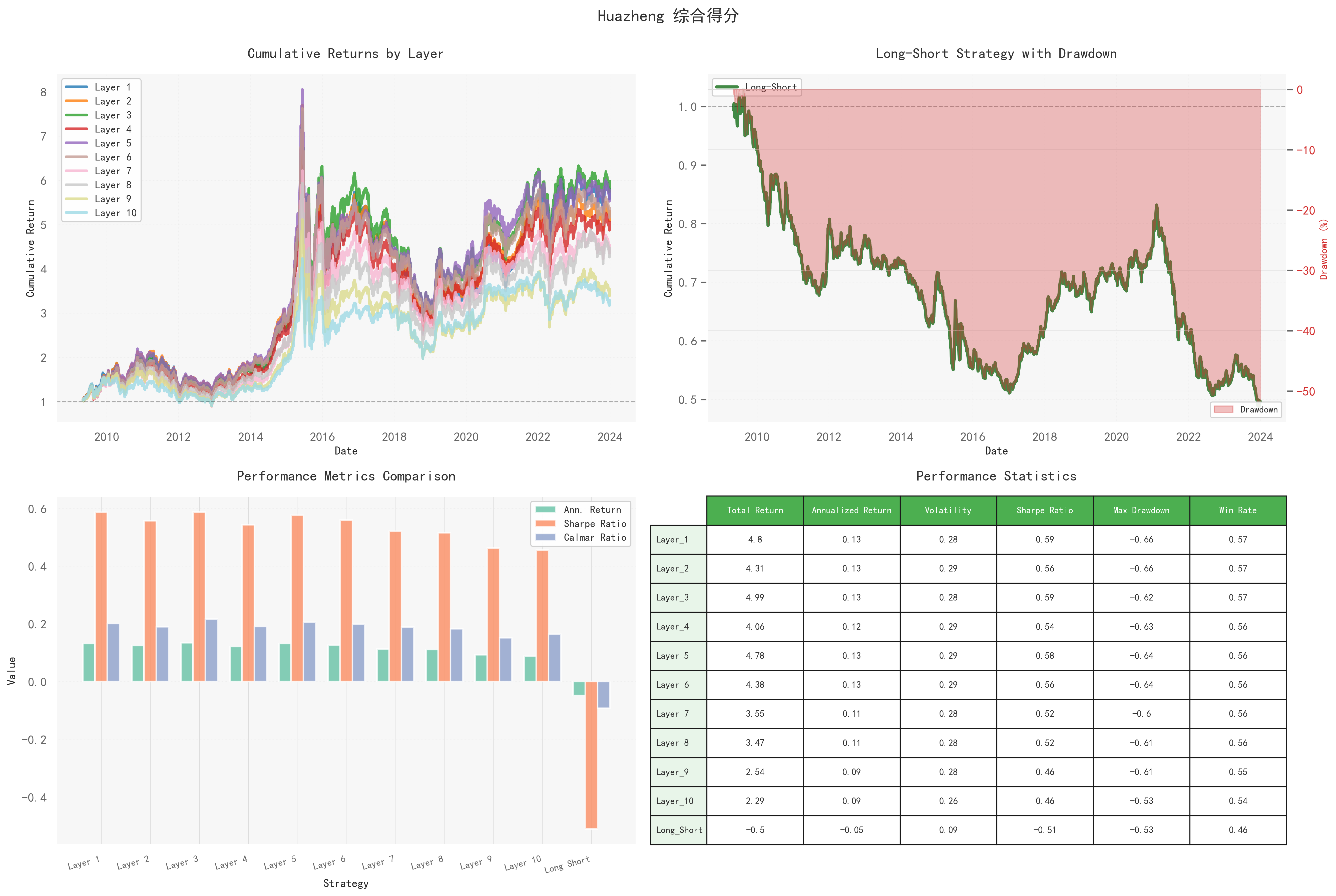
The net value trends of each layer are highly synchronized, showing no significant monotonic increasing feature. This means that a higher ESG score does not necessarily imply higher returns.
During the market bubble period of 2014–2015, all layers rose synchronously before falling back, indicating that this indicator reflects overall market style or cyclical fluctuations rather than serving as an independent source of excess returns.
The long-short portfolio (long high scores, short low scores) shows a long-term downward trend, with cumulative drawdowns approaching 50%, annualized returns around -0.05, and negative Sharpe ratios, indicating that the strategy is ineffective over the sample period.
From a performance perspective, annualized returns for each layer range between 0.09–0.13, with Sharpe ratios concentrated between 0.5–0.6, showing certain defensive stability.
4.2 Huazheng E Score
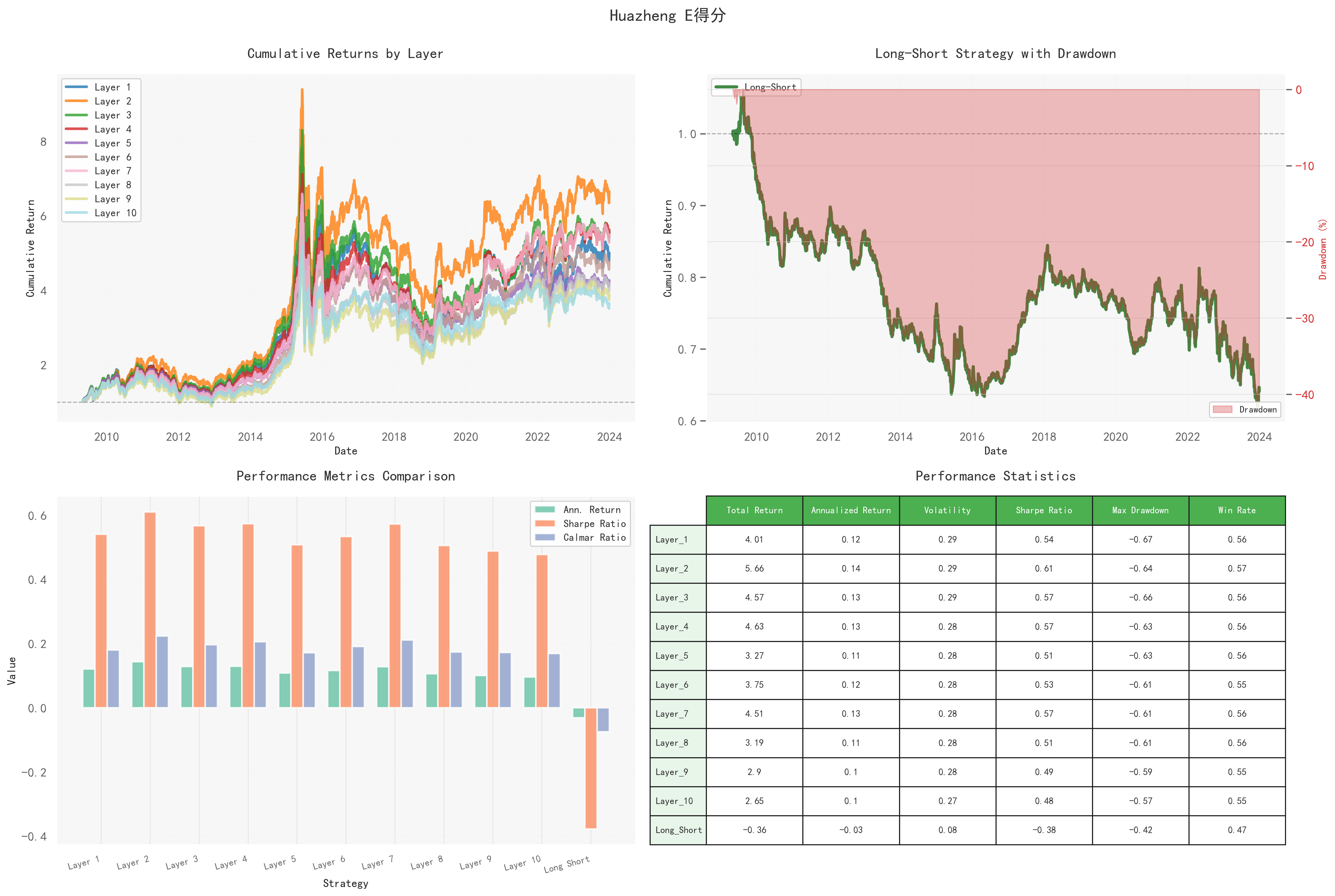
The E score shows slight differentiation across layers but does not form a stable monotonic relationship. Only a few medium-to-high score groups perform slightly better in specific periods.
The long-short net value continues to weaken from the beginning, with annualized returns around -0.03 and negative Sharpe ratios. Volatility across layers ranges between 0.27–0.29, and drawdown magnitudes are also similar.
The results indicate that the impact of environmental scores largely depends on policy or industry prosperity windows, lacking sustained excess return capability.
4.3 Huazheng S Score
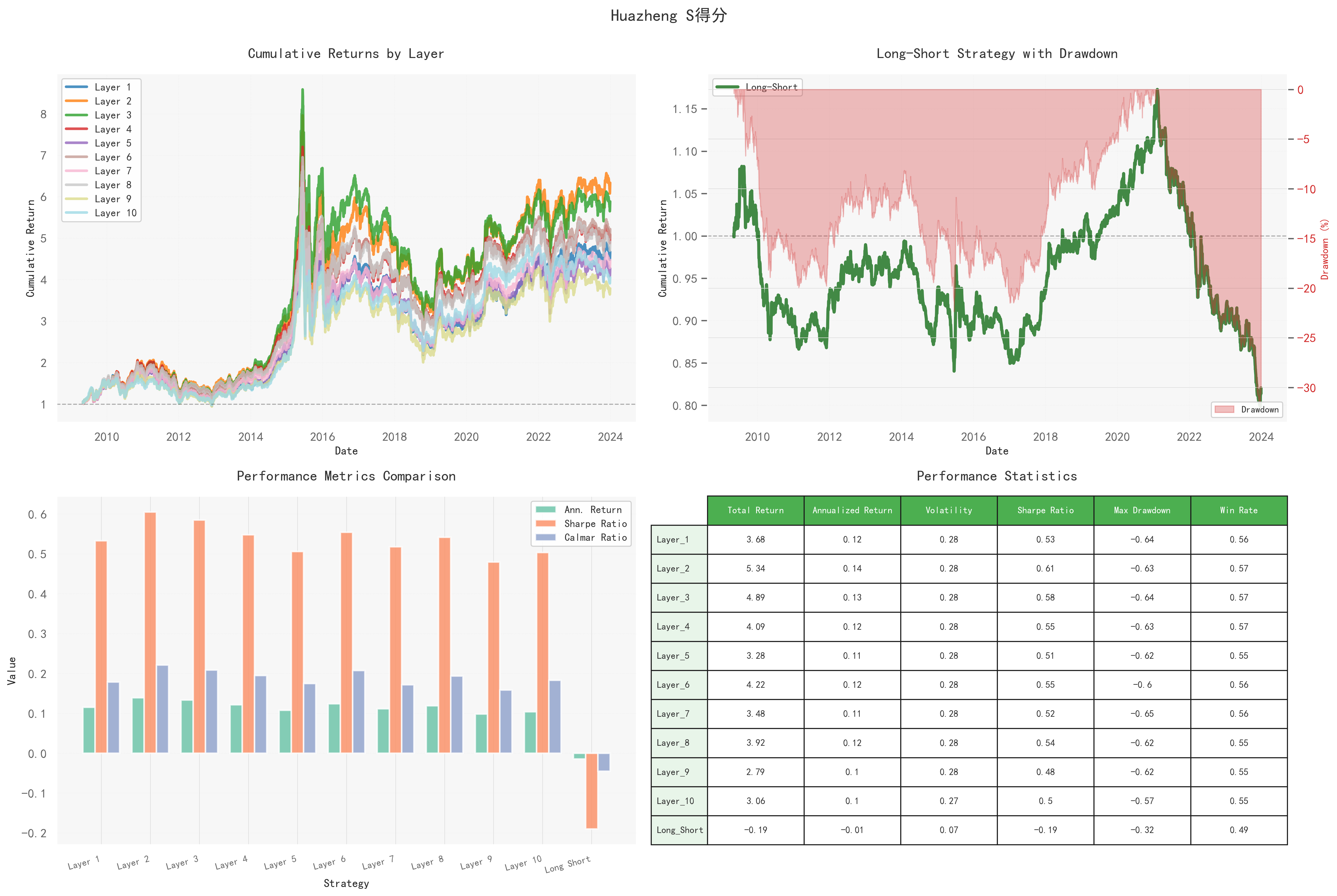
The net values for social score layers remain highly synchronized. Mid-range layers occasionally perform better, but the overall ranking is unstable.
The long-short strategy yields slightly negative returns long-term, with annualized returns around -0.01 and deep drawdowns, indicating that the "long high social scores, short low social scores" strategy lacks a profitable foundation.
Overall performance is close to that of the comprehensive score and E score. While its defensive attribute is slightly weaker than that of the G score, it still holds some advantage over an unfiltered benchmark, though the effect is limited.
4.4 Huazheng G Score
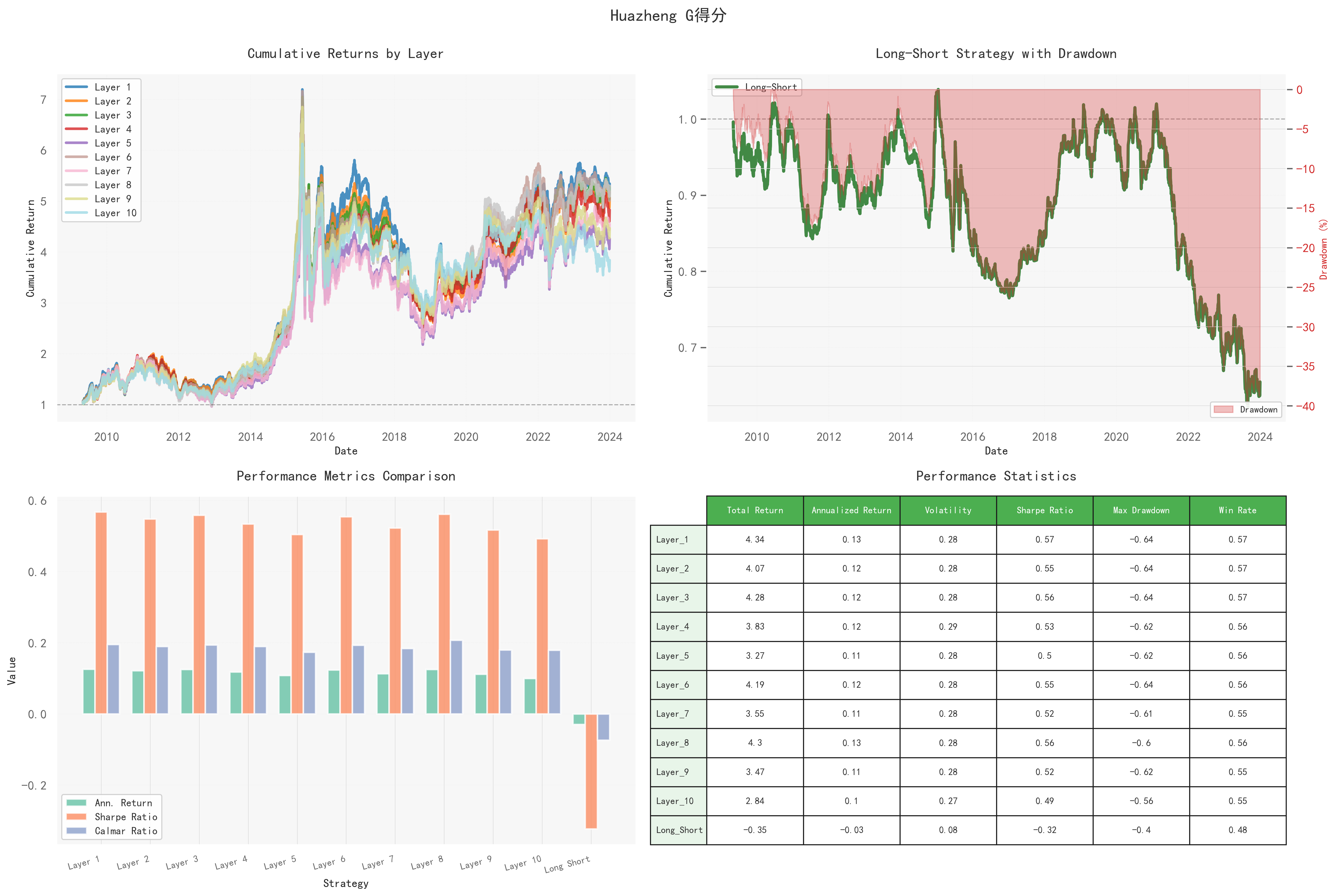
The governance score also does not present a stable monotonic return relationship. Its volatility and drawdown control are the most regular among the four score types, exhibiting characteristics similar to a low-volatility factor.
The long-short net value continues to decline, with annualized returns around -0.03 and negative Sharpe ratios, confirming that the "long good governance, short poor governance" strategy cannot穿越 cycles (withstand market cycles).
This score primarily reflects low volatility + low drawdown risk control characteristics, making it more suitable as a risk buffer unit in a portfolio rather than an offensive signal.
5. Comprehensive Comparison
The five charts give the same answer: ESG layering does not produce stable return rankings, and long-short positions are negative long-term; however, high layers are generally more "stable," with lower drawdowns and volatility. They can serve as risk constraints and low-volatility weights.
To obtain the complete code, you can subscribe to the "Quantide Research" platform membership. Platform introduction and payment methods are available at https://mp.weixin.qq.com/s/j1r-cH_3Agc7fz1WwGrYFQ