RSI Mean Reversion: Validating a Quantitative Trading Strategy

The Holy Grain Still Shines: Revalidating the RSI Strategy

The Holy Grail still shines. RSI remains my favorite indicator because tides and mean reversion are the life rings of this blue planet; such cycles also exist in the trading world. RSI is one of the best indicators for characterizing these market tides and reversion dynamics.

Earlier this year, I introduced Connor’s RSI. This time, we will explore a mean reversion strategy based on short-term RSI proposed by Larry Connors, focusing on how to approach strategy optimization.

Strategy experiments and evaluation data are sourced from Quantitativo.

---

Strategy Overview

Everyone should already be familiar with the RSI indicator. The RSI we commonly use is calculated based on 6, 12, and 24 periods.

$$ RS = \frac{\text{SMMA}(U,n)}{\text{SMMA}(D,n)} $$

$$ RSI = 100\cdot\frac{\text{SMMA}(U,n)}{\text{SMMA}(U,n) + \text{SMMA}(D,n)} = 100 - { 100 \over {1 + RS} } $$

However, Larry Connors argues that a 2-period RSI better reflects market trends and is likely the "Holy Grail" among technical indicators. He published this view in his 2008 book, Top Traders on Wall Street. In subsequent Connors RSI indicators, the RSI for streaks is indeed calculated using a 2-period window.

Based on this RSI, Connors proposed the following mean reversion strategy:

1. The S&P 500 index is above its 200-day moving average;
2. The 2-period RSI of the S&P 500 index is below 5;
3. When the signal is triggered, buy at the closing price;
4. Sell when the S&P 500 is above its 5-day moving average.

In trader terminology, this is a buy strategy during a bull market (index above the 200-day moving average) with a short-term pullback (RSI below 5).

---

Factor Testing

First, Quantitativo conducted a single-factor test. The methodology involved buying and holding all assets with a 2-day RSI closing below 5 for 5 days, then calculating the returns.

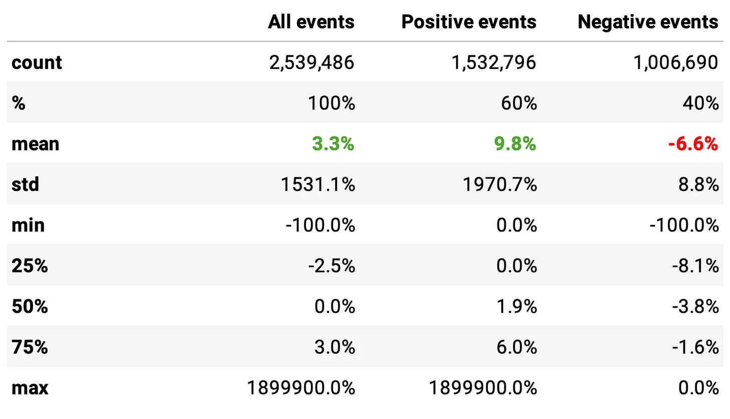
This statistic includes over 21,000 assets and more than 2.5 million events (S&P 500 closing above the 200-day moving average). Highlights from the test:

1. When any given stock’s 2-day RSI is below 5 and held for 5 days in a bull market, the average buy return is 3.3%;
2. 60% of events yield positive returns, with an expected return per trade of 9.8%;
3. 40% of trades are negative, with an expected return per trade of -6.6%;
4. The distribution is positively skewed.

---

Quantitativo also analyzed the reverse scenario: buying every stock when its 2-day RSI closes above 5 and holding for 5 days in a bull market. The results are:

1. When any given stock’s 2-day RSI is above 5, the expected buy return is 0.3%;
2. The probability of trades becoming positive is 52%, with an expected return of 5.5%;
3. The probability of trades becoming negative is 48%, with an expected return of -5.1%.

Quantitativo also performed a hypothesis test to determine if the two tests belong to the same distribution. The p-value was well below 0.05, proving that the two distributions are significantly different. Therefore, the factor in the first test contains Alpha.

Strategy Backtest

Next, Quantitativo conducted a strategy backtest. The strategy design is as follows:

1. Use SPY as the test asset.
2. Buy SPY at the next open when the following conditions are met:
   1. The S&P 500 index’s RSI(2) closes below 5.
   2. SPY is above its 200-day moving average.
3. Exit conditions:
   1. If SPY’s closing price is higher than the previous day’s high, exit at the next open.
   2. If SPY’s closing price falls below the 200-day moving average.

As you can see, the backtest strategy differs slightly from the one proposed by Connors. Why make such a differentiation?

---

The differentiation here reflects the gap between backtesting and live trading. Connors’ strategy is more idealized, whereas Quantitativo’s verification strategy is closer to live trading realities. This is a consideration we must always have when developing strategies.

First, although we can backtest using the S&P 500 index, a more practical approach in live trading is to purchase the corresponding ETF. Here, SPY is the ETF tracking the S&P 500.

Second, Connors’ strategy involves buying at the closing price. If your backtesting system is not precise enough, it is better to buy at the next day’s opening price. Of course, if your backtesting system and market data are precise to the minute level, in China, you can also calculate signals using the closing price one minute before the call auction and then buy during the call auction.

The difference in exit conditions can be viewed as an optimization by Quantitativo on the original strategy. However, I do not see the significance of this optimization. It seems to lack any underlying trading principle support. It looks more like overfitting derived from data by Quantitativo.

So, what were Quantitativo’s experimental results?

---

The test on SPY was simply a disaster. Over the entire backtest period (25 years), trading this strategy with SPY yielded a 67% return. The main reason is the low number of trades, executing only 157 transactions.

Next, Quantitativo switched to the Nasdaq 100 Index ETF (QQQ) and the 3x Leveraged Nasdaq 100 ETF (TQQQ). The results showed that TQQQ performed well:

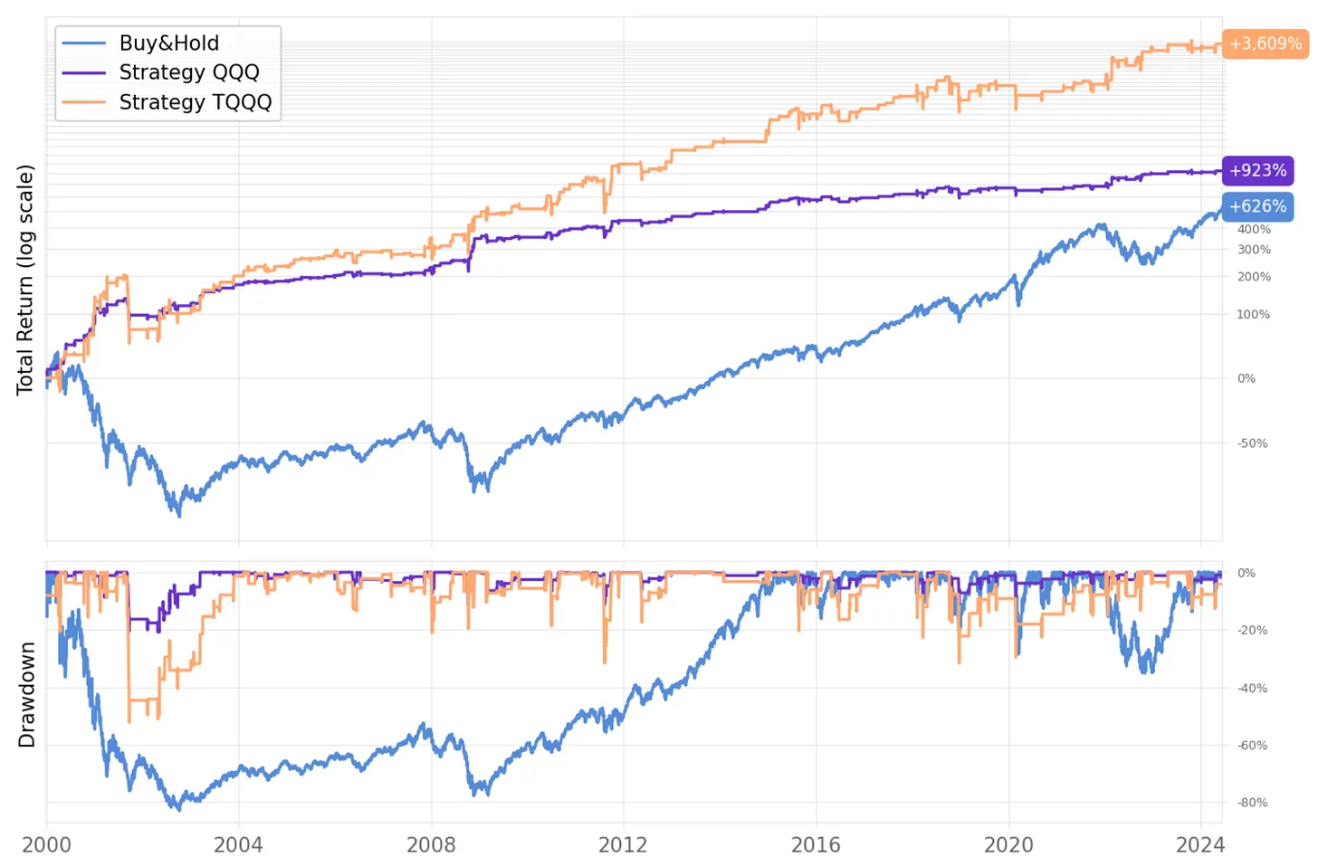
The Sharpe ratios reached 2.3 (QQQ) and 1.92 (TQQQ), which are quite good indicators for index assets (especially when compared to China A-shares).

---

Improved Strategy: Adding Factors

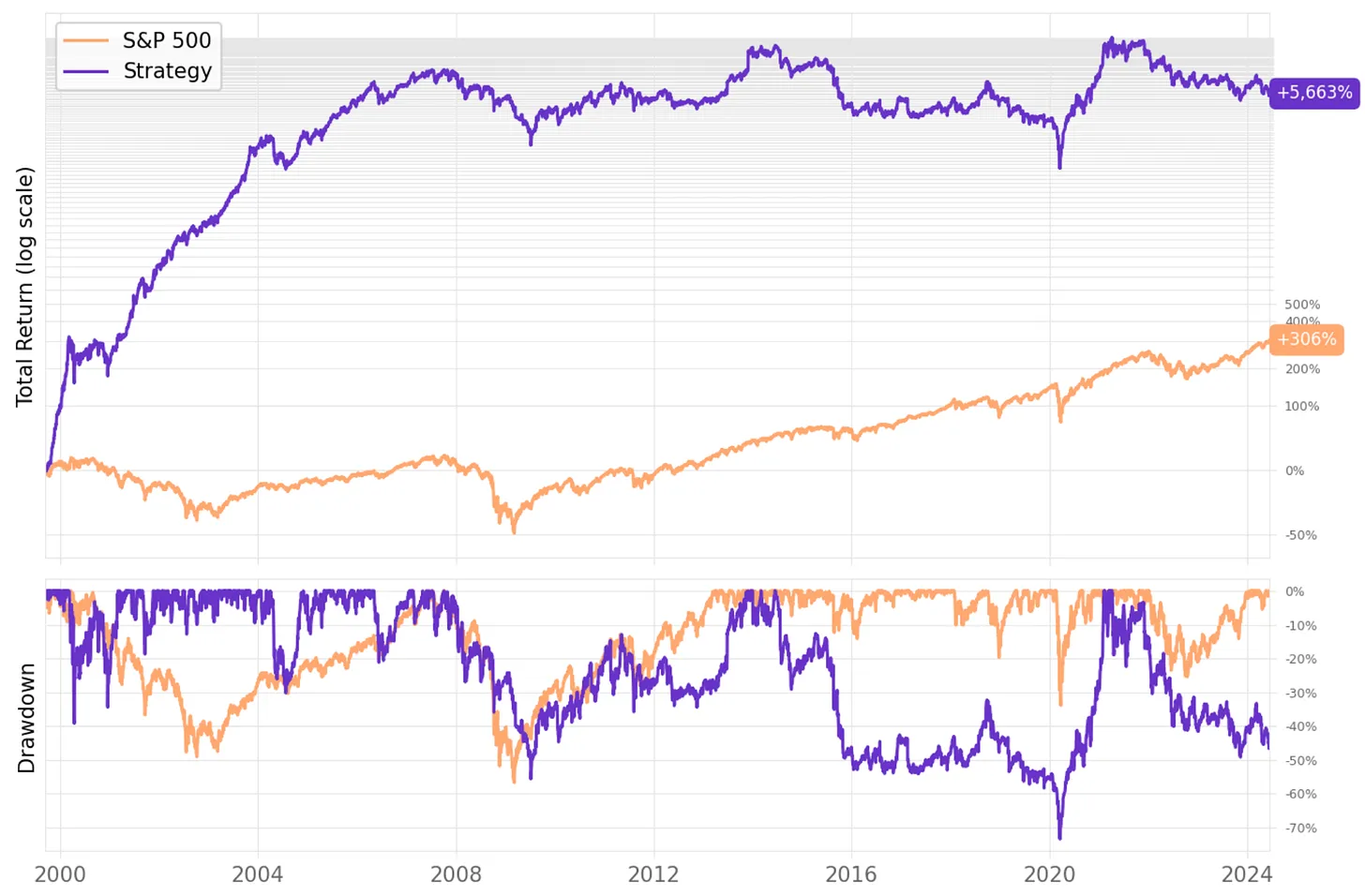
Building on the previous experiment, Quantitativo expanded the portfolio.

They divided the capital into ten slots (10 slots) to buy assets whose RSI closed below 5 the previous day; if the universe contains more than 10 assets triggering the entry signal, they are ranked by market cap, prioritizing smaller-cap stocks. The exit condition was changed to the closing price falling below the asset’s 200-day moving average.

Additionally, they restricted trading to assets with good liquidity:

1. Only trade assets that have not been suspended for the past 3 months.
2. Exclude assets if their median daily trading volume over the past 3 months is less than 20 times the capital slot size.

---

This time, the results were quite good, with an overall annual return of 17.8%, three times that of the benchmark. However, there is a problem: all of this was achieved in the first 8-9 years. The strategy stopped executing after 2008 and has since underperformed the benchmark.

Why? By analyzing the 11,380 trades executed during the 25-year backtest, Quantitativo found many delistings. The flaw in this naive approach is that the strategy prioritizes small-cap stocks (after passing the liquidity filter), which have a delisting probability of +70%.

Second Improvement: Reducing Delisting Risk

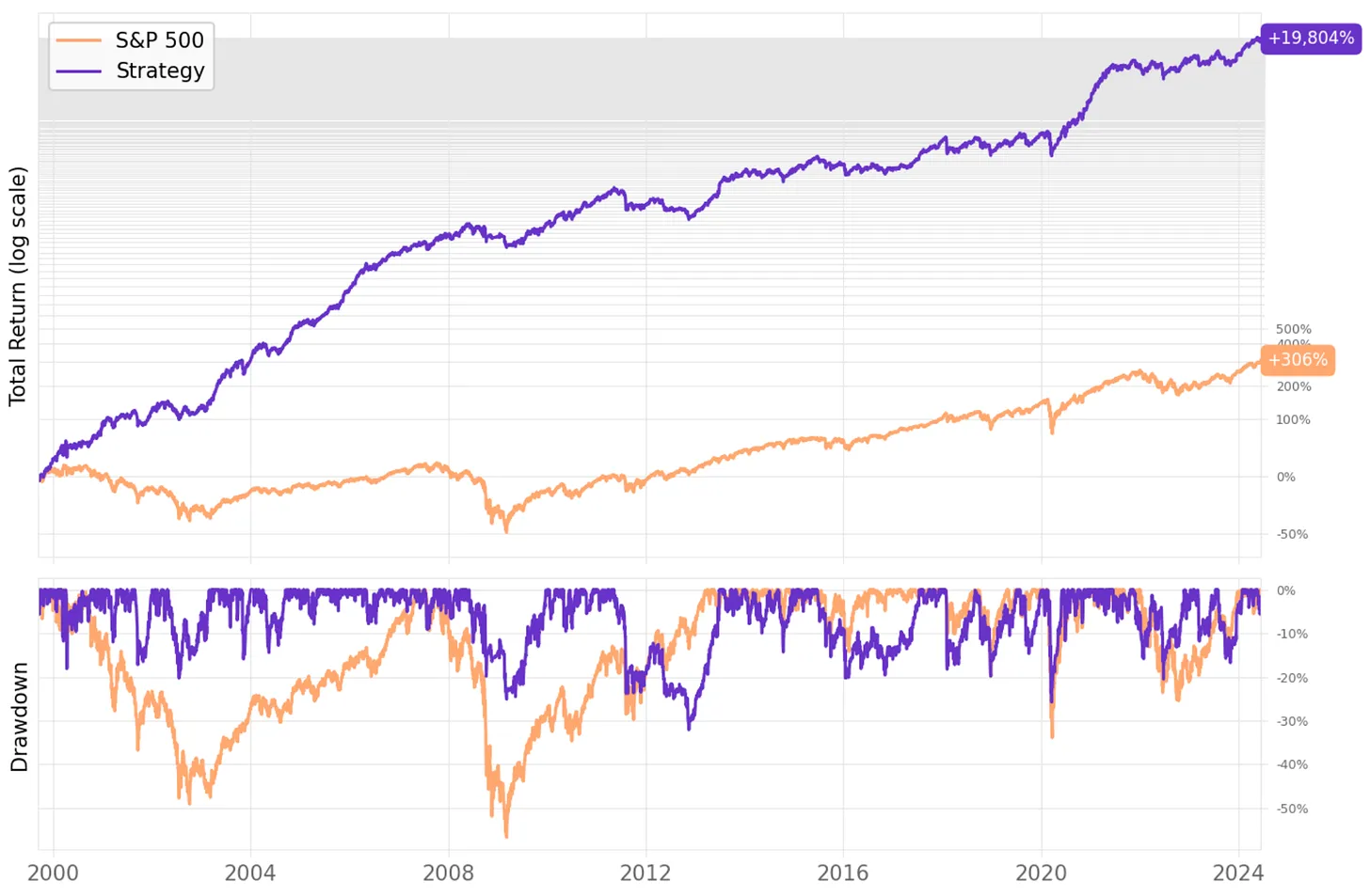
Quantitativo improved the strategy again, this time limiting the universe to trade only large-cap and mega-cap stocks, which have lower delisting probabilities (35% and 9%, respectively).

This time, the effect was significant. The strategy’s annualized return reached 23.9%, four times that of the benchmark during the same period, with a Sharpe ratio of 1.23 and a max drawdown of 32%, almost half that of the S&P 500.

However, a pre-existing problem remains: the number of trades is still too high. There are still 461 trades per year.

---

Third Improvement: Reducing Slots

The previous experiments used 10 slots, which was likely the main cause of the excessive number of trades. Thus, Quantitativo reduced the number of simultaneously held assets to 2.

Now, the number of trades has dropped from 461 per year to 90 per year, achieving an annual return of 30.3%, five times that of the benchmark.

Here is a question: Does the annualized return increase, and will the Sharpe ratio follow? Giving yourself more time to think is better than blindly accepting others' viewpoints. Therefore, I will not reveal the answer here. You can ask me in the comments or search for the answer on the Quantitativo website.

---

Conclusion

This article introduces a mean reversion strategy based on short-term RSI and, finally, presents an implementation with an annualized return of 30.3% (excluding slippage and transaction fees).

The core of this strategy is short-term RSI. Although this indicator was invented over 45 years ago, the backtest results show that if you study something deeply enough, you are likely to succeed.

This solution is worth your reading time, but more importantly, we discussed the general process of strategy discovery and optimization angles. Let’s recap as the closing remarks for this article:

1. RSI represents tides and mean reversion, rooted in human nature, so it will never go out of style.
2. Multi-factor strategies can also focus on one factor, introducing others as constraints during trading.
3. The article provides a method for judging asset liquidity, which you can also use as a factor.
4. The steps for developing strategies often start with single-factor testing, followed by simple backtesting, and then step-by-step optimization based on backtest results.
5. In the optimization process, Quantitativo first used ETFs, then switched to 10 slots, and finally returned to a 2-slot solution.