
Delivery-Day Curse: Why A-Shares Fell on March 27
Sunday's terrorist attack in Moscow put every China A-shares trader on edge — would A-shares have to foot the bill again? Sure enough, in just three days, the Shanghai Index lost 1.8% and the CSI 1000 fell 5.89%, with most investors losing money.
After the pain, a few questions are worth reviewing. First: what caused the fall? Of course, we tackle it the quant way.
The Delivery-Day Curse?
The most widely accepted explanation is that today is ETF options delivery day. On the previous delivery day, February 28, the Shanghai Index plunged 1.91%.
For reference, here are this year's key delivery dates:
| Month | Stock Index Futures | ETF Options | A50 |
|---|---|---|---|
| Jan | Jan 19 | Jan 24 | — |
| Feb | Feb 23 | Feb 28 | Feb 28 |
| Mar | Mar 15 | Mar 27 | Mar 28 |
| Apr | Apr 19 | Apr 24 | — |
| May | May 17 | May 22 | May 30 |
| Jun | Jun 21 | Jun 26 | Jun 27 |
| Jul | Jul 19 | Jul 24 | — |
| Aug | Aug 16 | Aug 21 | Aug 29 |
| Sep | Sep 20 | Sep 25 | Sep 27 |
| Oct | Oct 18 | Oct 23 | — |
| Nov | Nov 15 | Nov 20 | Nov 28 |
| Dec | Dec 20 | Dec 25 | Dec 30 |
Stock index futures expire on the third Friday of each month; ETF options expire on the Wednesday of the fourth week; A50 expires on the second-to-last trading day of the relevant month.
As quant researchers (or quant developers), we should be able to calculate these delivery dates ourselves.
tip
In our 24-lesson quant course, this problem appears as an exercise (with a reference answer). Here is the thinking behind the solution.calendar.monthcalendar(2024, 2)This returns the following:
| Monday | Tuesday | Wednesday | Thursday | Friday | Saturday | Sunday |
|---|---|---|---|---|---|---|
| 0 | 0 | 0 | 1 | 2 | 3 | 4 |
| 5 | 6 | 7 | 8 | 9 | 10 | 11 |
| 12 | 13 | 14 | 15 | 16 | 17 | 18 |
| 19 | 20 | 21 | 22 | 23 | 24 | 25 |
| 26 | 27 | 28 | 29 | 0 | 0 | 0 |
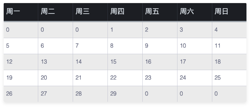
Zeros mean the day falls outside the current month. So to get every Friday, just convert the output above to a DataFrame and take the Friday column to get all Fridays. Then check whether the third Friday is a trading day — if not, take the fourth Friday.
Morgan Stanley's Prediction
Another rumor was an unverified Morgan Stanley note claiming that since the rebound to 3,090, A-shares had gained more than 15%, enough to lock in full-year 2024 profit expectations.
That was most likely false — apart from today, both Morgan Stanley and JPMorgan were adding to positions all week.
Trend Analysis
In our 24-lesson quant course, we cover several trend-analysis tools. With them, there is no need to guess the direct trigger for the plunge; in fact, recent price action had already flagged downside risk, and subsequent tests confirmed the downtrend was in place.
First, pressure at the 3,100 round number. In our article Left-Digit Effect: Round Numbers and Light Refraction, we introduced the left-digit effect and round-number support/resistance. Last Tuesday and Thursday confirmed that resistance was there.
Second, RSI analysis. The daily RSI peaked on February 23, then printed bearish top divergences on March 5, March 11 and March 18. The 30-minute RSI corrected several times in between, but at 10:00 on March 21 it diverged bearishly again. As taught in the course, an RSI move up to or above its prior high is a topping signal worth watching — if moving averages are flat or sloping down at the time, the top is essentially confirmed.
How do you find the prior RSI high? Our approach is to use the zigzag library to locate the previous high of the 5-day moving average; the RSI at that point is the prior high. The next time RSI approaches or exceeds that value, it is often a local top. Why not use zigzag to find the current high directly? Because zigzag needs several periods of delay to confirm a pivot. If we apply it to a moving average, the lag is even longer — by the time zigzag confirms the latest high, the best trading window is usually gone. By watching whether RSI is approaching its prior high instead, we can fire a signal immediately and then confirm in the next bar whether price action validates it.
Here is how to find local highs with zigzag:
from zigzag import peak_valley_pivots
close = ...
ma = moving_average(close, 5)
pct_change = ma[1:]/ma[:-1] - 1
std = np.std(pct_change)
up_thresh, down_thresh = 2*std, -2*std
peak_valley_pivots(ma, up_thresh, down_thresh)peak_valley_pivots requires two threshold parameters to confirm whether a local extreme counts as a peak or valley. Only when a point stands above both sides by more than up_thresh / down_thresh is it confirmed as a peak. Valleys are confirmed the same way.
Here we use a small statistical trick: twice the standard deviation of recent changes as the threshold.
If a point sits more than two standard deviations from the mean, it is indeed an outlier — geometrically, a peak or a valley. We have seen the same idea in Bollinger Bands or in seaborn envelope plots.
In the vast majority of cases, this method finds past peaks and valleys very accurately:
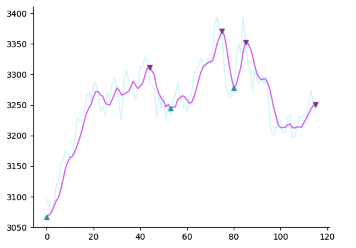
With these peaks and valleys, we can locate the previous RSI high and low. When RSI approaches that value again, we fire a signal and check signal quality in the next bar.
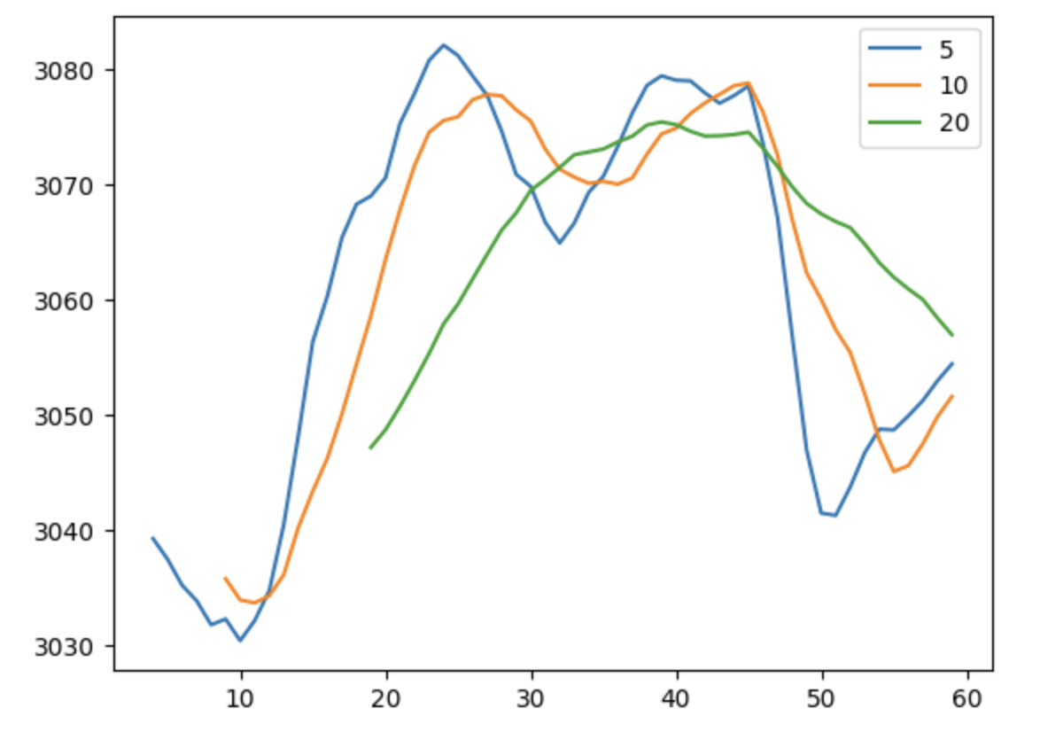
Finally, judging a moving-average turn. After 10:00 last Friday, the 20-period MA on the 30-minute chart had turned down, with price trading below it. Combined with the round-number resistance and the RSI high, it was time to cut exposure immediately.

Then at 14:00 on March 25, three 30-minute bars in a row failed to break back above the declining MA, confirming the rebound had failed. The 20-period line was pressing down like a roof. We call this MA pressure dome pressure. Some classic technical analysis fits it as a parabola. In the 24-lesson course, we introduce a more robust way to judge MA direction. After all, polynomial fitting is unusable in most cases.
Testing Signal Effectiveness
The round number, dome pressure and prior RSI high discussed here are all precisely defined and fully quantifiable. Readers can verify their effectiveness themselves.
You may ask: if these methods work, don't they amount to a money-printing machine?
In reality, the money printer is far more complex. Everyone knows the trick; execution is what differs. To track these signals in real time, you need a stable, high-performance quant framework.
Second, these tools work better for index-level analysis, but investing ultimately comes down to single stocks. Index analysis only pays off if you can pick stocks highly correlated with the market.
Moreover, even though we use multiple methods to front-run signals, there is still a lag from signal to confirmation. That makes both our exits and bottom-fishing a little late, giving up some profit. If the trend flips back and forth, lost profit plus trading costs can still lead to failure. Still, it clearly helps us avoid major losses.
Quant analysis does not guarantee you will be right 100% of the time, but it ensures that when you should be right, you are more likely to be right than others.
Global Asset Allocation
When a decline in A-shares looks confirmed, we should exit promptly. Cross-border ETFs are also worth considering. That has been especially clear in this year's market. For example, when the Shanghai Index started to rebound at 14:00 today, a cross-border ETF fell 1.6% from its high; and when the Shanghai Index pushed up into the 30-minute 20-period MA and was rejected at 14:15, the ETF immediately rebounded, rising 1.37% in the final half hour to close up 3.67%. At extreme moments, these cross-border ETFs seesaw against the Shanghai Index.