
Pandas: Counting Consecutive Daily Limits in China A-Shares

There are often scenarios where we need to quickly identify the strongest and weakest stocks over a specific period to analyze the characteristics of momentum and mean-reversion stocks within that interval.
If we rely on loops, it’s akin to counting on our fingers—something Ivy League graduates would likely disdain. So, let’s explore how to implement this functionality concisely and elegantly, while also showing off a bit of zhuangbility (showing off) to our colleagues.
We will use 2023 data as an example. The goal is to identify stocks that hit the daily price limit for $n$ consecutive days or more, and to record the dates of these limits. The same approach can also be used to find the weakest stocks and their corresponding timeframes.
You can copy the code below and verify it with your own data. However, if you are short on time, consider joining my community:

Members of the community will receive a Quantide research environment account, allowing you to run and download this tutorial directly.
First, let’s load the data:
np.random.seed(78)
start = datetime.date(2023,1,1)
end = datetime.date(2023, 12, 31)
barss = load_bars(start, end, -1)
barss.tail()The load_bars function is available in our research environment. This yields data in the following format:
| date | asset | open | high | low | close | volume | amount | price |
|---|---|---|---|---|---|---|---|---|
| 2023-12-25 | **** | 30.85 | 31.20 | 30.06 | 30.08 | 3591121.00 | 109649397.62 | 30.14 |
| 2023-12-26 | **** | 30.14 | 30.25 | 26.00 | 27.85 | 9042296.00 | 251945474.00 | 27.90 |
| 2023-12-27 | **** | 27.90 | 28.89 | 27.18 | 28.89 | 5488847.00 | 155156381.16 | 28.58 |
| 2023-12-28 | **** | 28.58 | 29.85 | 28.44 | 29.20 | 5027247.00 | 147201133.00 | 29.25 |
| 2023-12-29 | **** | 29.25 | 30.14 | 29.25 | 29.66 | 3923048.00 | 116933800.77 | NaN |
We extract only the price data and pivot it into a wide-format table to calculate the daily return signs:
pd.options.display.max_columns = 6
returns = barss.close.unstack("asset").pct_change()
returns.tail()This yields the following result:
| date | **** | **** | **** | ... | **** | **** | **** |
|---|---|---|---|---|---|---|---|
| 2023-12-25 | -0.00 | -0.01 | -0.02 | ... | -0.01 | -0.03 | -0.03 |
| 2023-12-26 | -0.01 | -0.01 | -0.02 | ... | 0.00 | -0.02 | -0.07 |
| 2023-12-27 | 0.00 | 0.00 | 0.02 | ... | -0.01 | 0.00 | 0.04 |
| 2023-12-28 | 0.04 | 0.03 | 0.01 | ... | 0.03 | 0.02 | 0.01 |
| 2023-12-29 | -0.01 | -0.01 | 0.02 | ... | 0.00 | -0.00 | 0.02 |
5 rows × 5085 columns
Next, we determine which days constitute a daily price limit. Since our objective is research rather than live trading, we can tolerate some approximation. We use the following logic to identify price limits (excluding stocks from the Beijing Stock Exchange and ST stocks):
criteria = ((returns > 0.095) & (returns < 0.105)) |
((returns > 0.19)& (returns < 0.21))
zt = returns[criteria].notna().astype(int)Key syntax points here include combining multiple conditions and converting NaN values to 0 while converting other values to 1.
NaN values appear because we are working with a wide-format table. In this format, some columns do not meet the condition at a specific point (row), while other columns do. To preserve the row, the non-meeting columns must be retained as NaN. We then use notna() to convert NaN to False and other values to True, finally casting them to integers 0 and 1, where 1 indicates a daily price limit occurred.
Next, we count the consecutive days of price limits for each asset using the following function:
def process_column(series):
g = (series.diff() != 0).cumsum()
g_cumsum = series.groupby(g).cumsum()
result = series.copy()
result[g_cumsum > 1] = g_cumsum[g_cumsum > 1]
return resultThe cleverness of this function lies in calculating the difference between each row and the previous row, followed by a cumulative sum. Consider the sequence: 0 0 1 1 1 0 0. The diff result is NaN, 0, 1, 0, 0, -1, 0. Non-zero values in diff indicate a change in the consecutive state: either the start of consecutive price limits or their termination.
By applying cumsum to the difference sequence, we establish a mapping with the original sequence:
| Original Sequence | diff | diff!=0 | cumsum |
|---|---|---|---|
| 0 | NaN | true | 1 |
| 0 | 0 | false | 1 |
| 1 | 1 | true | 2 |
| 1 | 0 | false | 2 |
| 1 | 0 | false | 2 |
| 0 | -1 | true | 3 |
| 0 | 0 | false | 3 |
If we treat cumsum as group identifiers, we can use groupby to calculate the count of non-zero values within each group, yielding the number of consecutive price limits. This corresponds to the operation in line 4.
Marvelous!
Finally, we apply this function:
df_processed = zt.apply(process_column, axis=0)
df_processed.stack().nlargest(5)We obtain the following (partial) results:
| date | asset | Consecutive Limits |
|---|---|---|
| 2023-10-25 | ******.XSHG | 14 |
| 2023-10-24 | ******.XSHG | 13 |
| 2023-03-21 | ******.XSHE | 12 |
| 2023-10-23 | ******.XSHG | 12 |
| 2023-03-20 | ******.XSHE | 11 |
Let’s verify one of these cases:
code = "******.XSHG"
bars = barss.xs(code, level="asset")
bars["frame"] = bars.index
plot_candlestick(bars.to_records(index=False),
ma_groups=[5,10,20,60])Here is the candlestick chart:
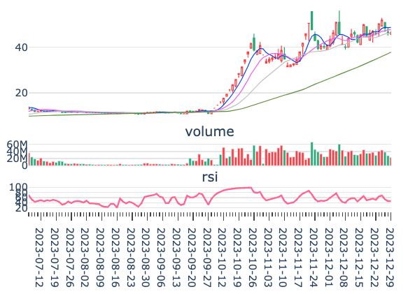
Lastly, let’s encapsulate the function:
def find_buy_limit(closes, low = 0.095, high = 0.105,n=50):
def process_column(series):
group = (series.diff() != 0).cumsum()
group_cumsum = series.groupby(group).cumsum()
result = series.copy()
result[group_cumsum > 1] = group_cumsum[group_cumsum > 1]
return result
returns = closes.unstack("asset").pct_change()
criteria = (returns > low) & (returns < high)
zt = returns[criteria].notna().astype(int)
df_processed = zt.apply(process_column, axis=0)
return df_processed.stack().nlargest(n)
find_buy_limit(barss.close)And finally, the Oscar goes to... the main force behind... (well, let’s not reveal even historical data).
When you don’t know where to kick, kick it into the goal! Now, go find patterns in the 14 consecutive price limits you missed last year!