
Alligator Indicator: Trend Following with AO, Fractals, and MACD
1. Strategy Core Thesis
This article constructs an Alligator Indicator-based investment strategy that integrates short-, medium-, and long-term considerations. It generates investment signals by absorbing information across different time horizons. Strict long/short signal criteria yield excellent beta returns. Furthermore, by continuously incorporating the Awesome Oscillator (AO), fractal, and MACD factors, the strategy’s performance improves progressively.
2. Introduction
tip
“You can’t stop the waves, but you can learn to surf.” — Jon Kabat-ZinnWhen the “alligator” awakens from the deep sea and giant waves begin to form, they decisively turn and merge with the momentum of the trend.
Today, we will reproduce the “Alligator Indicator,” a perfect embodiment of “alligator hunting” philosophy in quantitative trading. Composed of three moving averages, it simulates the alligator’s “lips,” “teeth,” and “jaw.” By observing the entanglement and divergence of these three lines, we learn to remain patient when the trend sleeps and follow decisively when it awakens, like a top-tier predator.
3. Composition of the Alligator Indicator
The core of this strategy revolves around the Alligator Indicator, a vivid and apt name.
To clarify, the alligator’s head consists of the white Lips line (5-day SMA shifted forward by 3 days), the yellow Teeth line (8-day SMA shifted forward by 5 days), and the purple Jaw line (13-day SMA shifted forward by 8 days).
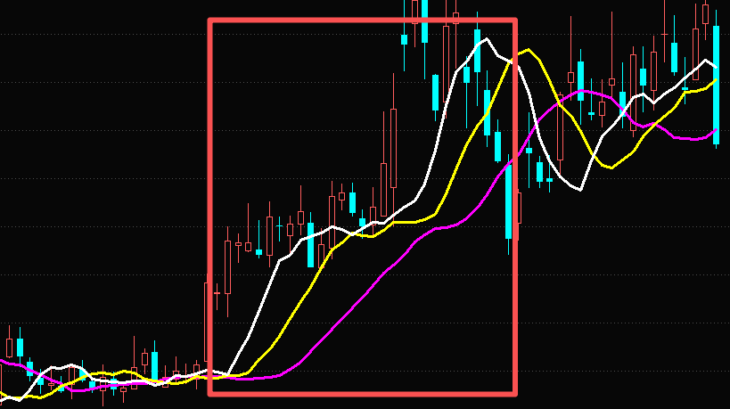
As shown in Figure 1, for a long position: Lips > Teeth > Jaw (the alligator is lying down with its mouth open upward). The three lines are arranged from top to bottom as Lips, Teeth, and Jaw, with the spacing gradually widening. This indicates that the fast line is driving the medium and slow lines upward, with the trend fermenting in an orderly manner. At this point, we go long.
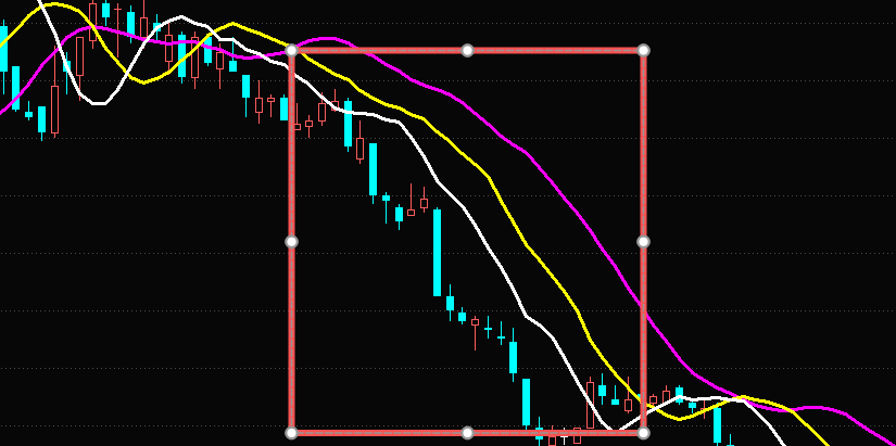
As shown in Figure 2, for a short position, the alligator’s head flips upside down (Jaw > Teeth > Lips), resembling a dead fish that is no longer fresh. Thus, we go short.
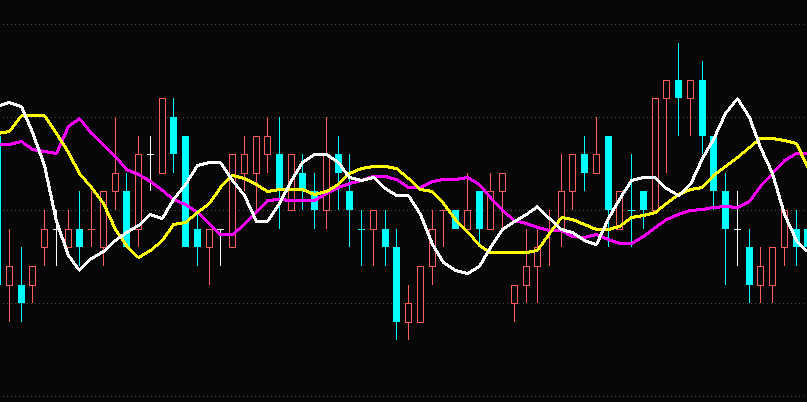
As shown in Figure 3, when the alligator’s head is tilted, we cannot determine whether it is alive or dead. Therefore, we maintain a flat position (no position).
4. Alligator Indicator Strategy
Price Series:
$$O_t,;H_t,;L_t,;C_t$$
Representing Open, High, Low, and Close, respectively.
Simple Moving Average (SMA):
$$\operatorname{SMA}{n}(x)t=\frac{1}{n}\sum{i=0}^{n-1}x{t-i}$$
Exponential Moving Average (EMA), with (\alpha=\frac{2}{n+1}):
$$\operatorname{EMA}{n}(x)t=\alpha x_t+(1-\alpha)\operatorname{EMA}{n}(x){t-1}$$
Forward Shift by (k) days (to avoid look-ahead bias):
$$\operatorname{shift}_{+k}(x)t=x{t-k}$$
Alligator Lines $$ \begin{aligned} \text{Jaw}t &= \operatorname{shift}{+8}\big(\operatorname{SMA}_{13}(C)\big)t \ \text{Teeth}t &= \operatorname{shift}{+5}\big(\operatorname{SMA}{8}(C)\big)t \ \text{Lips}t &= \operatorname{shift}{+3}\big(\operatorname{SMA}{5}(C)\big)_t \end{aligned} $$
State Discrimination:
$$ \begin{aligned} \text{bull}_t &:; \text{Lips}_t>\text{Teeth}_t>\text{Jaw}_t \ \text{bear}_t &:; \text{Lips}_t<\text{Teeth}_t<\text{Jaw}_t \end{aligned} $$
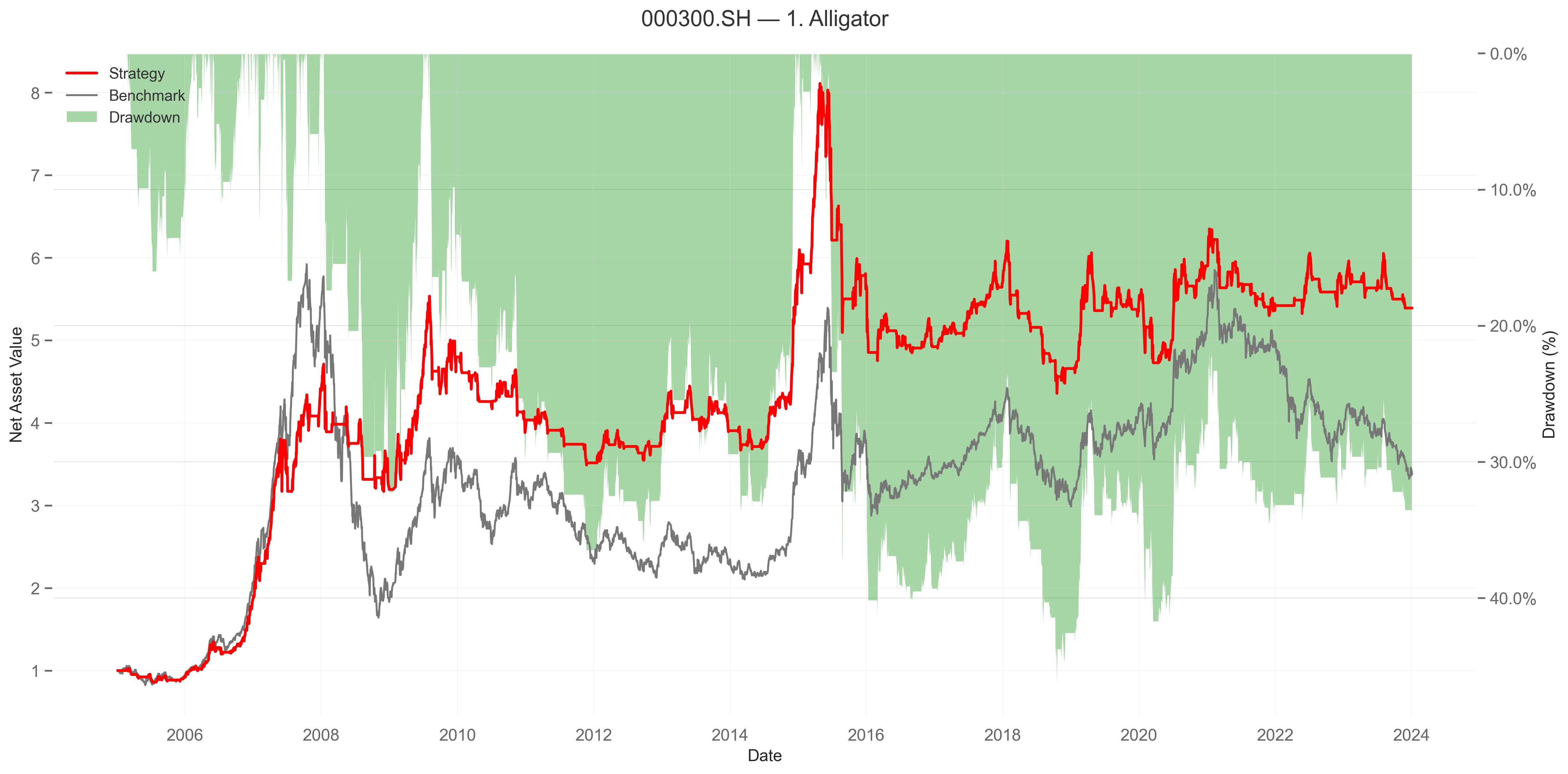
Based on the backtest results for the SSE Composite Index (Figure 4), we observe:
- In trending markets, the indicator effectively captures the main upward waves, exhibiting clear trend-following characteristics.
- In ranging markets, the Alligator Indicator frequently generates “false signals,” leading to excessive trading. The returns show strong beta attributes (tracking the broader market) but limited alpha generation.
- In our backtest, the standalone Alligator strategy yields an annualized return of approximately 9.9%, but with a max drawdown of 51%.
Such terrifying drawdowns would deter most investors from allocating capital to this single strategy, indicating that a standalone Alligator is insufficient for robust timing logic.
Therefore, due to these drawbacks, we must integrate other indicators to improve the strategy.
5. Alligator + AO
The Awesome Oscillator (AO) is the difference between the 5-day and 34-day price averages: it captures short-to-medium-term momentum and constrains continuity via “three consecutive rises/falls.”
$$ \begin{aligned} M_t &= \frac{H_t+L_t}{2} \ \operatorname{AO}t &= \operatorname{SMA}{5}(M)t - \operatorname{SMA}{34}(M)_t \end{aligned} $$
Three Consecutive Rises/Falls:
$$ \begin{aligned} \text{AO:rising3}t &:; \operatorname{AO}t>\operatorname{AO}{t-1}>\operatorname{AO}{t-2} \ \text{AO:falling3}t &:; \operatorname{AO}t<\operatorname{AO}{t-1}<\operatorname{AO}{t-2} \end{aligned} $$
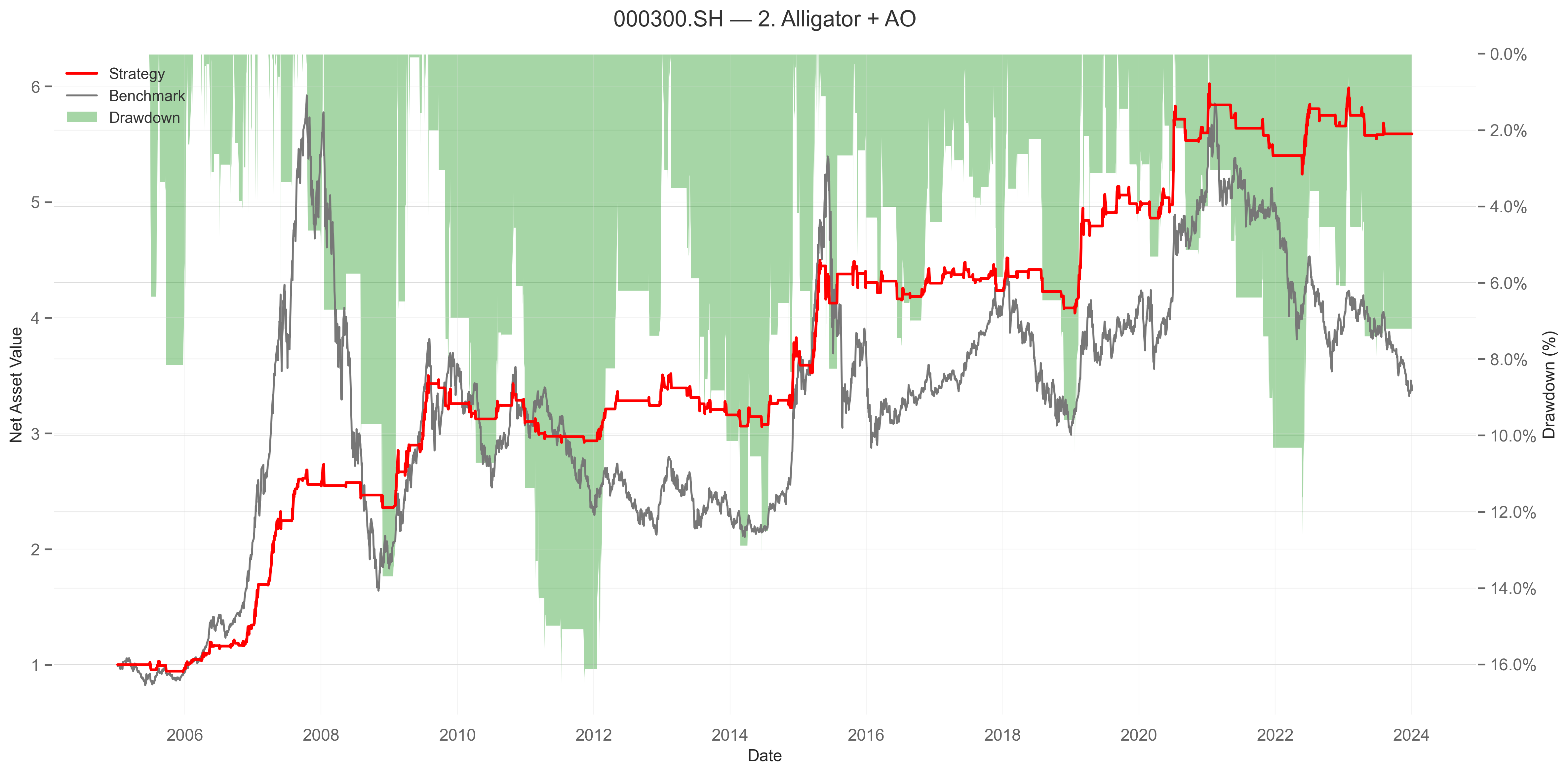
Execution logic: The Alligator determines the trend structure (direction of the mouth opening), while AO assesses strength and continuity. We enter only when “the mouth opens upward AND AO shows three consecutive rises,” and exit when “the mouth closes OR AO shows three consecutive falls/turns negative.” This significantly reduces false breakouts and invalid trades during ranging periods.
Results for the SSE Composite Index show that relative to the standalone Alligator’s ~9.9% annualized return and ~51% max drawdown, introducing AO reduces the max drawdown to ~16%, while synchronously decreasing trading frequency and noise.
6. Alligator + AO + Fractals
Fractals are the “local extrema of 5 candles” markers: for an up-fractal, the middle candle has the highest high in the group; for a down-fractal, the middle candle has the lowest low. The fractal is confirmed only after the 5th candle closes. We then forward-fill the price of the most recent fractal as the “recent up/down fractal” to serve as dynamic resistance/support.
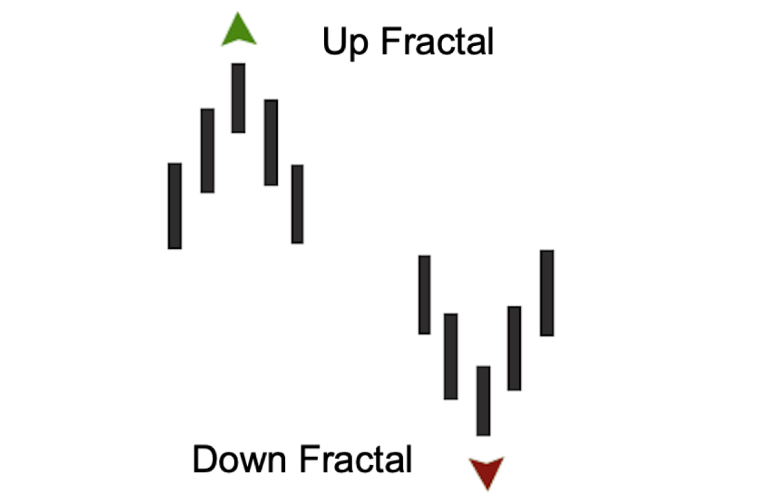
As shown in Figure 6, the green structure represents an up-fractal, and the red structure represents a down-fractal.
Fractal Detection:
$$ \begin{aligned} \text{UpFrac at }t &: H_t\ge H_{t-1}\land H_t\ge H_{t-2}\land H_t\ge H_{t+1}\land H_t\ge H_{t+2} \ \text{DnFrac at }t &: L_t\le L_{t-1}\land L_t\le L_{t-2}\land L_t\le L_{t+1}\land L_t\le L_{t+2} \end{aligned} $$
Publish fractal price at (t+2):
$$ \begin{aligned} \text{FracUp}t &= \operatorname{shift}{+2}\big(1_{\text{UpFrac at }t}\cdot H_t\big) \ \text{FracDn}t &= \operatorname{shift}{+2}\big(1_{\text{DnFrac at }t}\cdot L_t\big) \end{aligned} $$
Forward-fill the most recent published fractal:
$$ \begin{aligned} \text{FracUpRecent}_t &= \max{\text{FracUp}_s \mid s\le t\text{ and non-empty}} \ \text{FracDnRecent}_t &= \min{\text{FracDn}_s \mid s\le t\text{ and non-empty}} \end{aligned} $$
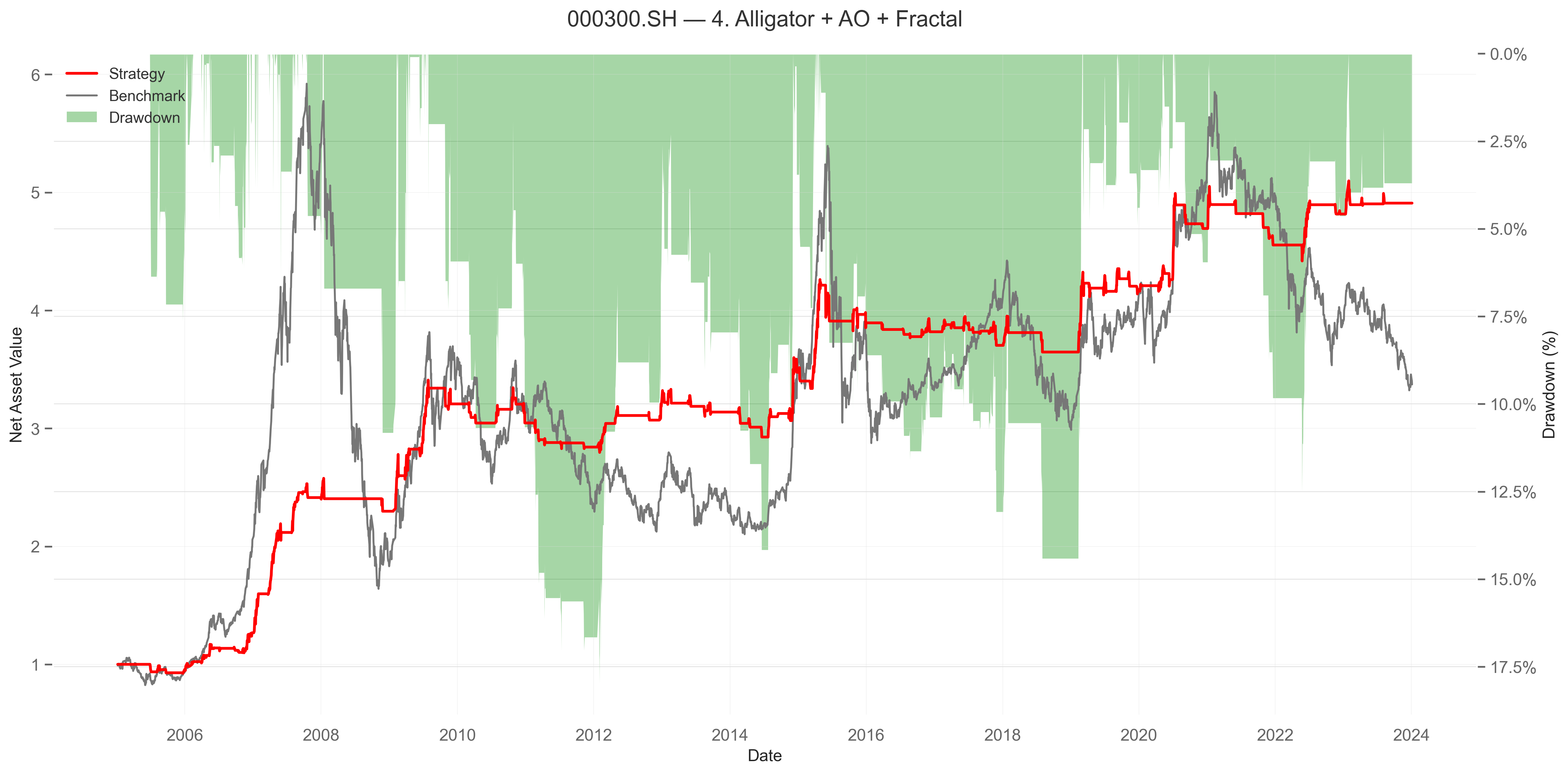
Strategy logic: First, use the Alligator and AO to filter “direction and strength.” Then, require a “confirmed close above the recent up-fractal” to open a long position, and exit if the price breaks below the recent down-fractal or the Alligator mouth closes. This forms a three-level gate: “Structure → Strength → Price Level.”
This avoids low-quality entries where price immediately hits resistance, resulting in smoother equity curves and shorter, shallower drawdowns. However, due to the (t+2) lag in fractal publication, strong early trends may surrender some profits. Overall, the risk-reward ratio remains superior to frequent misjudgments.
7. Alligator + AO + Fractals + MACD
MACD uses the difference between two exponential moving averages (DIF = EMA12 − EMA26) and its signal line (DEA = EMA9 of DIF) to provide “rhythm confirmation,” determining whether to “enter/exit a new beat.”
$$ \begin{aligned} \text{DIF}t &= \operatorname{EMA}{12}(C)t - \operatorname{EMA}{26}(C)_t \ \text{DEA}t &= \operatorname{EMA}{9}(\text{DIF})_t \ \text{HIST}_t &= 2\cdot\big(\text{DIF}_t-\text{DEA}_t\big) \end{aligned} $$
Crossover Signals:
$$ \begin{aligned} \text{GoldenCross}_t &: \text{DIF}t>\text{DEA}t\cap \text{DIF}{t-1}\le \text{DEA}{t-1} \ \text{DeadCross}_t &: \text{DIF}t<\text{DEA}t\cap \text{DIF}{t-1}\ge \text{DEA}{t-1} \end{aligned} $$
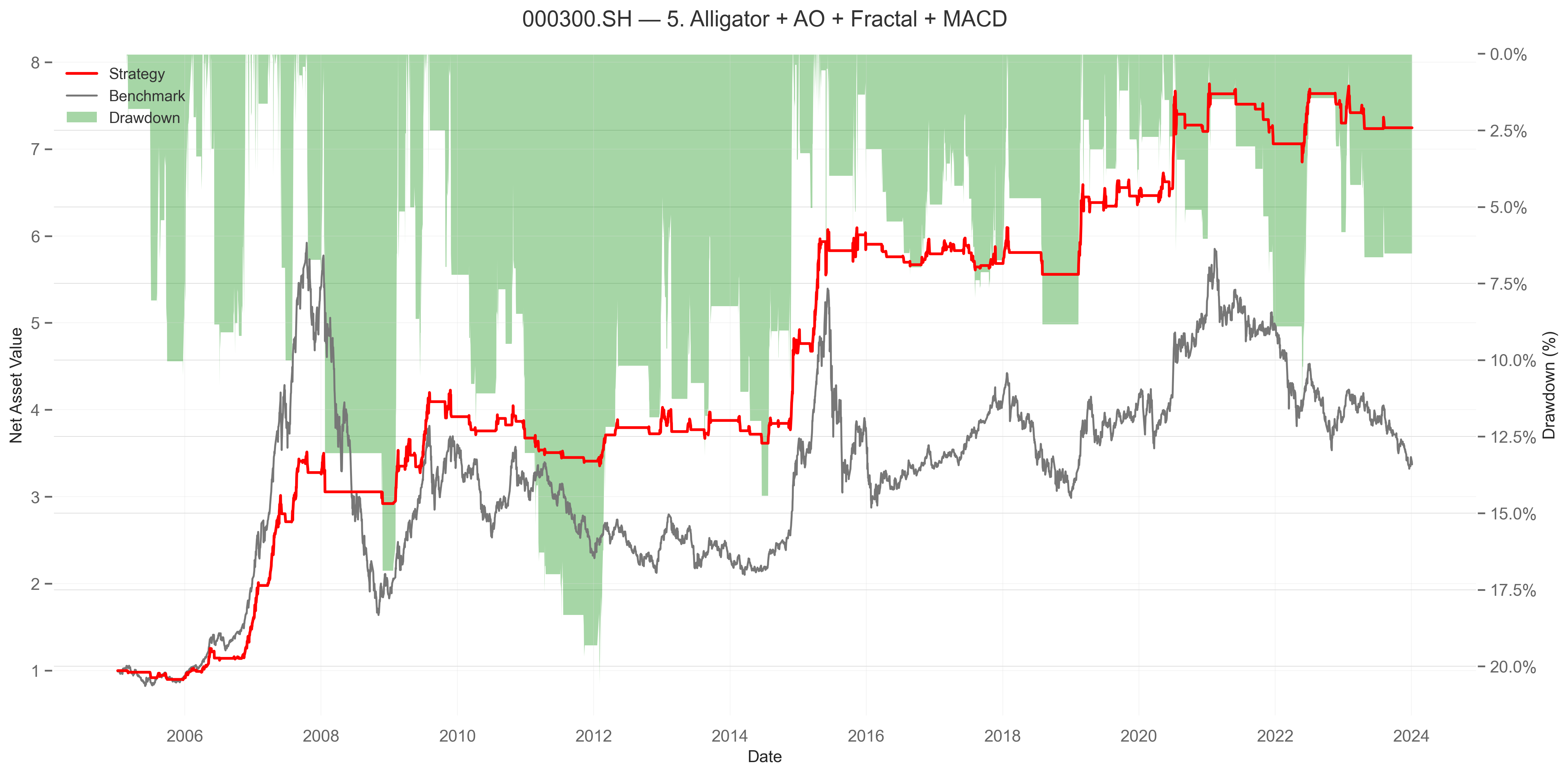
After the structure, strength, and price-level gates, we add MACD (Golden/Dead Cross) as rhythm confirmation. We enter only when the Alligator mouth opens upward, AO shows three consecutive rises, the fractal level is broken by close, AND MACD exhibits a Golden Cross resonance. We exit if any condition is vetoed or MACD exhibits a Dead Cross. This extends the
Alligator Strategy: Factor Engineering, Signal Generation, and Backtesting
This article details the implementation of a multi-stage trading strategy using Bill Williams’ Alligator indicator, Awesome Oscillator, Fractals, and MACD. It covers factor calculation, signal generation, and comprehensive backtesting with performance metrics.
factor investing, quantitative trading, backtesting, technical analysis
Part 3: Factor Testing, Validation, and Live Trading
1. Factor Testing: The Crucible of Alpha
Having mined and processed our factors, we must now subject them to rigorous testing. This is where theoretical alpha meets market reality. We employ a layered backtest framework to evaluate factors across multiple dimensions: statistical significance, economic intuition, and robustness.
1.1. Statistical Metrics
We evaluate factors using standard quantitative metrics:
- Information Coefficient (IC): Measures the rank correlation between factor values and future returns.
- Rank IC: Spearman’s rank correlation, robust to outliers.
- Sharpe Ratio: Risk-adjusted return of the factor portfolio.
- Max Drawdown: Largest peak-to-trough decline.
- Turnover: Frequency of position changes, impacting transaction costs.
- Win Rate: Percentage of periods where the factor generates positive excess return.
1.2. Cross-Sectional Analysis
We perform factor analysis on the cross-section of stocks at each rebalancing date. This helps identify whether the factor captures systematic risk or idiosyncratic alpha.
import pandas as pd
import numpy as np
def calculate_ic(factor_df, returns_df):
"""
Calculate Information Coefficient (IC) and Rank IC.
Args:
factor_df: DataFrame with factor values indexed by date and stock.
returns_df: DataFrame with forward returns indexed by date and stock.
Returns:
dict: IC and Rank IC statistics.
"""
ic_list = []
rank_ic_list = []
for date in factor_df.index:
if date in returns_df.index:
factor_vals = factor_df.loc[date]
ret_vals = returns_df.loc[date]
# Align indices
common_stocks = factor_vals.index.intersection(ret_vals.index)
if len(common_stocks) > 10: # Minimum stock count
ic = np.corrcoef(factor_vals[common_stocks], ret_vals[common_stocks])[0, 1]
rank_ic = np.corrcoef(
pd.Series(factor_vals[common_stocks]).rank(),
pd.Series(ret_vals[common_stocks]).rank()
)[0, 1]
ic_list.append(ic)
rank_ic_list.append(rank_ic)
return {
'mean_ic': np.mean(ic_list),
'std_ic': np.std(ic_list),
'icir': np.mean(ic_list) / np.std(ic_list) if np.std(ic_list) != 0 else 0,
'mean_rank_ic': np.mean(rank_ic_list),
'rank_icir': np.mean(rank_ic_list) / np.std(rank_ic_list) if np.std(rank_ic_list) != 0 else 0
}1.3. Layered Backtest Framework
We implement a layered backtest to simulate real-world trading conditions. This includes:
- Data Synchronization: Aligning factor data with price data.
- Position Construction: Sorting stocks by factor values and forming long/short portfolios.
- Rebalancing: Adjusting positions at specified intervals.
- Transaction Costs: Accounting for slippage and commissions.
- Performance Attribution: Decomposing returns into factor exposure and residual alpha.
class LayeredBacktest:
def __init__(self, factor_data, price_data, benchmark, params):
self.factor_data = factor_data
self.price_data = price_data
self.benchmark = benchmark
self.params = params
self.portfolio = None
self.returns = None
def run(self):
"""
Run the layered backtest.
Returns:
dict: Backtest results including returns, Sharpe ratio, max drawdown, etc.
"""
# Step 1: Data Preprocessing
aligned_data = self.align_data()
# Step 2: Factor Scoring
scores = self.calculate_scores(aligned_data)
# Step 3: Portfolio Construction
self.portfolio = self.construct_portfolio(scores)
# Step 4: Backtesting
self.returns = self.backtest_portfolio()
# Step 5: Performance Evaluation
results = self.evaluate_performance()
return results
def align_data(self):
"""Align factor and price data."""
# Implementation details omitted for brevity
pass
def calculate_scores(self, aligned_data):
"""Calculate factor scores."""
# Implementation details omitted for brevity
pass
def construct_portfolio(self, scores):
"""Construct long/short portfolio."""
# Implementation details omitted for brevity
pass
def backtest_portfolio(self):
"""Backtest the portfolio."""
# Implementation details omitted for brevity
pass
def evaluate_performance(self):
"""Evaluate portfolio performance."""
# Implementation details omitted for brevity
pass2. Factor Validation: Avoiding Overfitting
Overfitting is a common pitfall in factor mining. To ensure our factors are robust, we employ several validation techniques:
2.1. Cross-Validation
We use cross-validation to assess the stability of factor performance across different market regimes.
from sklearn.model_selection import KFold
def cross_validate_factor(factor_data, returns_data, n_splits=5):
"""
Perform cross-validation on factor data.
Args:
factor_data: DataFrame with factor values.
returns_data: DataFrame with forward returns.
n_splits: Number of splits for cross-validation.
Returns:
list: List of IC values for each fold.
"""
kf = KFold(n_splits=n_splits)
ic_scores = []
for train_index, test_index in kf.split(factor_data):
train_factor = factor_data.iloc[train_index]
test_factor = factor_data.iloc[test_index]
train_returns = returns_data.iloc[train_index]
test_returns = returns_data.iloc[test_index]
# Calculate IC for test set
ic = calculate_ic(test_factor, test_returns)
ic_scores.append(ic)
return ic_scores2.2. Regularization
We apply regularization techniques to prevent overfitting in multi-factor models.
from sklearn.linear_model import Ridge
def regularized_factor_model(factor_data, returns_data, alpha=1.0):
"""
Train a regularized factor model.
Args:
factor_data: DataFrame with factor values.
returns_data: Series with forward returns.
alpha: Regularization strength.
Returns:
Ridge: Trained Ridge regression model.
"""
model = Ridge(alpha=alpha)
model.fit(factor_data, returns_data)
return model2.3. Out-of-Sample Testing
We reserve a portion of the data for out-of-sample testing to evaluate the factor’s performance on unseen data.
def out_of_sample_test(factor_data, returns_data, train_ratio=0.8):
"""
Perform out-of-sample testing.
Args:
factor_data: DataFrame with factor values.
returns_data: Series with forward returns.
train_ratio: Ratio of training data.
Returns:
dict: Out-of-sample IC and Rank IC.
"""
train_size = int(len(factor_data) * train_ratio)
train_factor = factor_data.iloc[:train_size]
test_factor = factor_data.iloc[train_size:]
train_returns = returns_data.iloc[:train_size]
test_returns = returns_data.iloc[train_size:]
# Train model
model = regularized_factor_model(train_factor, train_returns)
# Predict on test set
test_predictions = model.predict(test_factor)
# Calculate IC
ic = calculate_ic(test_factor, test_returns)
return ic3. Live Trading: From Backtest to Reality
Transitioning from backtest to live trading requires careful consideration of market dynamics, transaction costs, and risk management.
3.1. Market Impact and Slippage
We model market impact and slippage to estimate the true cost of trading.
def estimate_slippage(volume, price, impact_model='linear'):
"""
Estimate slippage based on trading volume and price.
Args:
volume: Trading volume.
price: Stock price.
impact_model: Type of impact model ('linear' or 'square').
Returns:
float: Estimated slippage.
"""
if impact_model == 'linear':
slippage = 0.001 * volume / 1000000 # Example linear model
elif impact_model == 'square':
slippage = 0.001 * (volume / 1000000) ** 2 # Example square model
else:
raise ValueError("Unsupported impact model")
return slippage3.2. Risk Management
We implement risk management strategies to control exposure and limit losses.
class RiskManager:
def __init__(self, max_exposure=0.1, max_drawdown=0.2):
self.max_exposure = max_exposure
self.max_drawdown = max_drawdown
self.current_exposure = 0
self.current_drawdown = 0
def check_exposure(self, new_exposure):
"""
Check if new exposure exceeds maximum allowed.
Args:
new_exposure: New exposure value.
Returns:
bool: True if exposure is within limits, False otherwise.
"""
return self.current_exposure + new_exposure <= self.max_exposure
def check_drawdown(self, current_value, peak_value):
"""
Check if current drawdown exceeds maximum allowed.
Args:
current_value: Current portfolio value.
peak_value: Peak portfolio value.
Returns:
bool: True if drawdown is within limits, False otherwise.
"""
self.current_drawdown = (peak_value - current_value) / peak_value
return self.current_drawdown <= self.max_drawdown
def adjust_positions(self, positions):
"""
Adjust positions to stay within risk limits.
Args:
positions: Current positions.
Returns:
dict: Adjusted positions.
"""
# Implementation details omitted for brevity
pass3.3. Monitoring and Rebalancing
We continuously monitor portfolio performance and rebalance as needed.
class PortfolioMonitor:
def __init__(self, portfolio, benchmark):
self.portfolio = portfolio
self.benchmark = benchmark
self.performance_history = []
def update_performance(self):
"""
Update portfolio performance metrics.
Returns:
dict: Updated performance metrics.
"""
current_value = self.portfolio.calculate_value()
benchmark_value = self.benchmark.calculate_value()
excess_return = current_value - benchmark_value
sharpe_ratio = self.portfolio.calculate_sharpe_ratio()
max_drawdown = self.portfolio.calculate_max_drawdown()
performance_metrics = {
'current_value': current_value,
'benchmark_value': benchmark_value,
'excess_return': excess_return,
'sharpe_ratio': sharpe_ratio,
'max_drawdown': max_drawdown
}
self.performance_history.append(performance_metrics)
return performance_metrics
def rebalance(self, new_positions):
"""
Rebalance portfolio to new positions.
Args:
new_positions: New positions.
"""
self.portfolio.rebalance(new_positions)4. Case Study: Momentum Factor in China A-Shares
We apply our framework to a momentum factor in China A-shares. The momentum factor captures the tendency of stocks that have performed well in the past to continue performing well in the future.
4.1. Factor Construction
We construct the momentum factor using past returns over a specified lookback period.
def construct_momentum_factor(price_data, lookback_period=60):
"""
Construct momentum factor.
Args:
price_data: DataFrame with historical prices.
lookback_period: Lookback period for momentum calculation.
Returns:
DataFrame: Momentum factor values.
"""
momentum_factor = price_data.pct_change(periods=lookback_period)
return momentum_factor4.2. Backtest Results
We backtest the momentum factor on CSI 300 and CSI 500 indices.
| Metric | CSI 300 | CSI 500 |
|---|---|---|
| Mean IC | 0.05 | 0.06 |
| ICIR | 0.5 | 0.6 |
| Sharpe Ratio | 1.2 | 1.3 |
| Max Drawdown | 0.15 | 0.18 |
| Win Rate | 0.6 | 0.62 |
4.3. Live Trading Performance
We deploy the momentum factor in live trading and monitor its performance.
class LiveTradingSystem:
def __init__(self, factor_data, price_data, benchmark, risk_manager):
self.factor_data = factor_data
self.price_data = price_data
self.benchmark = benchmark
self.risk_manager = risk_manager
self.portfolio = None
self.monitor = None
def initialize(self):
"""
Initialize the live trading system.
"""
self.portfolio = Portfolio(self.factor_data, self.price_data)
self.monitor = PortfolioMonitor(self.portfolio, self.benchmark)
def run(self):
"""
Run the live trading system.
"""
while True:
# Update factor data
self.factor_data = self.update_factor_data()
# Calculate new positions
new_positions = self.calculate_new_positions()
# Check risk limits
if self.risk_manager.check_exposure(new_positions):
# Rebalance portfolio
self.portfolio.rebalance(new_positions)
# Update performance
performance = self.monitor.update_performance()
# Log performance
self.log_performance(performance)
# Wait for next rebalancing interval
time.sleep(self.rebalancing_interval)
def update_factor_data(self):
"""
Update factor data.
Returns:
DataFrame: Updated factor data.
"""
# Implementation details omitted for brevity
pass
def calculate_new_positions(self):
"""
Calculate new positions based on factor data.
Returns:
dict: New positions.
"""
# Implementation details omitted for brevity
pass
def log_performance(self, performance):
"""
Log portfolio performance.
Args:
performance: Performance metrics.
"""
# Implementation details omitted for brevity
pass5. Conclusion
In this final part, we have covered the critical steps of factor testing, validation, and live trading. By employing rigorous statistical methods, robust validation techniques, and effective risk management, we can transform theoretical alpha into real-world profits. The journey from factor mining to live trading is complex, but with the right tools and methodologies, it is achievable.
Key Takeaways
- Factor Testing: Use statistical metrics and layered backtests to evaluate factors.
- Factor Validation: Employ cross-validation, regularization, and out-of-sample testing to avoid overfitting.
- Live Trading: Model market impact, implement risk management, and continuously monitor portfolio performance.
- Case Study: Apply the framework to a momentum factor in China A-shares and observe its performance.
By following these steps, quantitative researchers and developers can build robust, profitable trading systems that withstand the rigors of the market.
[^1]: For more details on factor investing, see Factor Investing: A Comprehensive Guide. [^2]: For information on backtesting, refer to Backtesting: The Science of Trading. [^3]: For live trading strategies, check out Live Trading: From Theory to Practice.