
Can Reinforcement Learning Evolve Trading Wisdom?
Content Summary
* Reinforcement learning (RL) is already used by J.P. Morgan and top global investment firms. * Unlike supervised learning, RL doesn't just accept standard answers at every step; it experiments and endures short-term losses to secure long-term gains, giving it the ability to withstand financial data noise. * The reward is the soul of RL. We can directly use portfolio return as the reward. In supervised learning, the loss function is core, but we cannot use return as a loss function. * This article includes complete, impressive RL code that does not depend on frameworks like FinRL and can run in the domestic market.In fact, RL has long had practical applications in quantitative investing. Although the flagship strategies of some top investment firms are kept secret, we have found cases indicating that top Wall Street players have already begun using RL.
For instance, around 2017, global top-tier investment bank J.P. Morgan launched LOXM1, a "shadow" trading execution platform. The "secret weapon" driving this platform is exactly our protagonist today—Reinforcement Learning (RL).
LOXM’s goal is clear: when executing large stock orders, it intelligently splits large orders into countless small ones, navigating complex market microstructures like a top trader, to complete transactions with the lowest impact cost and highest speed.
This is no longer simply predicting price movements; it is learning the art of "how to trade" within dynamic market博弈 (game theory).
What Exactly Is Reinforcement Learning?
So, what exactly is this high-sounding RL?
According to the article Reinforcement Learning for Quantitative Trading2, we can construct a unified framework to understand it.
Imagine you are playing an electronic game, and your goal is to score as high as possible. In this game:
- You are the Agent. In quantitative trading, this agent is your trading algorithm.
- The game world is the Environment. In trading, this is the rapidly changing financial market.
- The visuals and states you see in the game (e.g., your health, position, number of enemies) are the State. In trading, this can be stock prices, trading volume, technical indicators, macroeconomic data, etc.
- Every operation you press (move forward, backward, fire) is the Action. In trading, this corresponds to buying, selling, or holding.
- The score you gain or lose after each action is the Reward. In trading, this is usually the return or loss of your portfolio.
The core idea of RL is to let the Agent (trading algorithm) continuously "trial and error" (take actions) in the Environment (financial market), learning an optimal Policy based on the Reward (return or loss) obtained after each trial, thereby maximizing cumulative reward (long-term return) over the long term. It is not learning "what the market will do next second," but learning 'what is the optimal action given the current market state.'
Where Does RL Excel?
At this point, you might ask: we already have supervised learning (e.g., predicting stock price movements) and unsupervised learning (e.g., clustering to discover market styles), why do we need RL? Where exactly does it excel?
The fundamental difference between RL and supervised/unsupervised learning lies in the learning paradigm.
Supervised learning is like memorizing a book of standard answers. You give it a historical K-line chart (input features) and tell it whether the next day will rise or fall (label). It learns a static "pattern recognition" ability. Unsupervised learning, on the other hand, finds patterns in a pile of data without answers, such as automatically grouping similar stocks. They are all trying to answer "what is it?"
RL, however, learns a decision-making process. It has no "standard answer" to memorize. The market does not tell you "buying at this exact moment is the only correct answer." RL faces a series of decisions, each affecting future states and potential returns. It answers the question "what should be done?" This is a dynamic, causal, and future-oriented learning process.
Some might say, "I can use a supervised learning model and continuously train and predict with new data (i.e., online learning). What is the difference from RL?"
On the surface, both continuously adapt to new data, but their cores are completely different. RL’s core advantages lie in two dimensions that supervised learning cannot reach:
Exploration vs. Exploitation
This is the soul of RL. Imagine a restaurant you often visit that tastes good (exploitation), but you occasionally want to try a new place, just in case there’s a surprise (exploration)? RL agents balance between "executing known optimal strategies" and "trying unknown strategies that may have higher returns" during training. This spirit of exploration allows RL to potentially discover superior trading patterns that human traders or supervised learning models have never considered. Supervised learning would only tell you that, based on historical experience, going to that old restaurant is the "correct answer."Learning Dynamic Causality
RL focuses on the causal link between a sequence of actions (e.g., buy A first, then sell B) and the final result. It understands that sometimes a short-term loss (e.g., actively accepting floating losses to lower the cost basis for building a position) is for a larger long-term goal. Supervised learning looks at only one "time slice" at a time, making it difficult to understand this cross-time, delayed causal logic.Financial data is known for its low signal-to-noise ratio, filled with random fluctuations and "false signals." RL’s advantage in such environments stems primarily from its unique design:
Focus on Long-Term Returns, Tolerating Short-Term Pain: Supervised learning models pursue prediction accuracy at each time point. If market noise causes it to make an incorrect prediction, it is "punished." RL’s goal is to maximize the cumulative return of the entire trading process. This means it can consciously execute an action that looks like a loss in the short term (e.g., buying when it seems like the price is about to fall) if this action is part of its long-term winning strategy (e.g., judging it as a fake breakdown by main forces). This "delayed gratification" characteristic gives it stronger immunity to short-term market noise.
Dynamic Adaptation, Not Marking the Boat: Market styles shift; factors effective yesterday may be invalid today. Once trained, supervised learning models have relatively fixed patterns, like a fool marking the boat to find his sword. RL agents’ strategies are functions of the state; they are designed to dynamically adjust their behavior according to environmental changes. When the market shifts from a bull to a bear market, RL agents can perceive this change through continuous interaction with the environment and adjust their trading strategies accordingly, shifting from aggressive long positions to conservative or even short positions. This innate adaptability is key to combating non-stationary markets.
Starting from "Chasing Gains and Cutting Losses" AlphaStock
Top-tier institutional quantitative strategies are kept secret. Even for public models like J.P. Morgan’s LOXM, their construction and operational mechanisms remain inaccessible to ordinary people. So, as quantitative traders, how do we build our own RL trading models?
In 2019, a team from Tsinghua University and Microsoft Research Asia developed a model named AlphaStock3. This model cleverly combines RL with the Attention Mechanism (yes, the core of Transformer models) specifically to optimize an ancient yet effective strategy—chasing gains and cutting losses (i.e., momentum trading).
Traditional momentum strategies are simple: buy stocks that performed well in the past, sell those that performed poorly. But the question is, when does momentum persist? When does it reverse?
AlphaStock’s cleverness lies in not relying on fixed rules but letting the RL agent learn. The agent observes price and volume data for hundreds of stocks in the market (state) and decides how much capital to allocate to which stocks (action). If this decision brings positive returns in the future, it receives a positive reward; otherwise, it receives a negative one. Through backtesting and training on massive historical data, AlphaStock eventually learns how to dynamically identify and utilize momentum effects in the market, and even to some extent avoid the risk of momentum reversal. This is like a martial arts master who, through countless实战 (actual battles), eventually develops a keen intuition for the game situation.
The theory sounds beautiful, but how to put it into practice? Can we make a useful RL model ourselves? Next, I will demonstrate how to build an RL trading model.
Get Hands Dirty! Let’s Practice!
For those who can access yfinance and alpaca_trade_api "infinitely" (i.e., without restrictions), I strongly recommend starting with the FinRL open-source library. It is hailed as the "OpenAI Gym for finance," greatly lowering the entry barrier.
Installing FinRL
First, ensure you have a Python environment (recommended to create a virtual environment using Anaconda or venv), then install FinRL and its dependencies via pip.
pip install finrlHowever, FinRL depends on yfinance and alpaca_trade_api, and most of our readers may not be able to use these two libraries. In that case, you might have to use the Gymnasium library and do a bit more work.
tip
Gymnasium is the successor to OpenAI Gym, an open-source toolkit for developing and comparing reinforcement learning algorithms. It provides standardized environment interfaces, allowing researchers and developers to test algorithm performance more conveniently.If we don’t use FinRL, we need to install two reinforcement learning libraries with strange names.
tip
The term "Gymnasium" comes from the Ancient Greek word "γυμνάσιον" (gymnasion), literally meaning "a place for naked exercise." In modern English, it often refers to a gym. In German, it also refers to a middle school.Among these two libraries, Gym is the interface, while SB3 provides various algorithms. In our example, we will use the PPO algorithm it provides. Below is the guide to installing these two libraries.
pip install gymnasium
pip install stable_baselines3Next, we need to obtain data. This part has no much nutritional value, so we won’t show the code to avoid taking up too much of your reading time. You can use any data source you like; ultimately, you need to get a DataFrame with data and asset as dual indexes, and column names must at least include: open, high, low, close, volume.
In the example, we will use cached data. If you want to run this example locally, you can obtain data via Tushare.
def get_stock_data_tushare(asset_list, start_date, end_date):
"""使用 tushare 获取股票数据(兼容方法,返回与 load_bars 相同格式)"""
all_data = []
# 转换日期格式为字符串
start_str = start_date.strftime("%Y%m%d")
end_str = end_date.strftime("%Y%m%d")
for asset in asset_list:
try:
# 获取日线数据
df_stock = pro.daily(ts_code=asset, start_date=start_str, end_date=end_str)
if not df_stock.empty:
# 重命名列以匹配 load_bars 格式
df_stock = df_stock.rename(
columns={"trade_date": "date", "vol": "volume"}
)
# 转换日期格式
df_stock["date"] = pd.to_datetime(df_stock["date"])
# 添加 asset 列
df_stock["asset"] = asset
# 按日期排序(tushare 返回的数据是倒序的)
df_stock = df_stock.sort_values("date").reset_index(drop=True)
# 选择需要的列
df_stock = df_stock[
["date", "asset", "open", "high", "low", "close", "volume"]
]
all_data.append(df_stock)
print(f"成功获取 {asset} 的数据,共 {len(df_stock)} 条记录")
else:
print(f"警告:{asset} 没有数据")
except Exception as e:
print(f"获取 {asset} 数据时出错:{e}")
if all_data:
# 合并所有股票数据
df_combined = pd.concat(all_data, ignore_index=True)
# 设置双重索引以匹配 load_bars 格式
df_combined = df_combined.set_index(["date", "asset"]).sort_index()
return df_combined
else:
return pd.DataFrame()How to Get the Code for This Article?
If you don’t want to write code, you can enroll in our course *Factor Mining and Machine Learning Strategies* to get runnable examples. This example can run completely locally.warnings.filterwarnings("ignore")
参数设置
N_STOCKS = 50 # 股票数量,可以调整进行多次随机测试 DATA_START_DATE = datetime.date(2010, 1, 1) DATA_END_DATE = datetime.date(2021, 10, 31)
数据划分比例 (train:test)
TRAIN_RATIO = 0.8
In quantitative trading, we have never seen an end-to-end AI model succeed. Basically, we always start with feature engineering before building machine learning models. Therefore, next, we need to create a `FeatureEngineer` class to handle feature engineering.
```python
class FeatureEngineer:
def __init__(self, use_technical_indicator=True, tech_indicator_list=None):
self.use_technical_indicator = use_technical_indicator
self.tech_indicator_list = tech_indicator_list or [
"macd",
"rsi",
"sma",
"bbands",
]
def preprocess_data(self, df):
df_reset = df.reset_index()
processed_stocks = []
for asset in df_reset["asset"].unique():
stock_data = df_reset[df_reset["asset"] == asset].copy().sort_values("date")
# 检查是否有足够的有效数据
if stock_data["close"].dropna().empty:
print(f"⚠️ 跳过股票 {asset}:没有有效的价格数据")
continue
# 前向填充价格数据,处理停牌等情况
price_columns = ["open", "high", "low", "close"]
for col in price_columns:
if col in stock_data.columns:
# 仅使用历史信息前向填充,避免后向填充引入未来价格
stock_data[col] = stock_data[col].ffill()
# 成交量用 0 填充(停牌时成交量为 0 是合理的)
if "volume" in stock_data.columns:
stock_data["volume"] = stock_data["volume"].fillna(0)
close = stock_data["close"].values.astype(float)
if "macd" in self.tech_indicator_list:
macd, macd_signal, macd_hist = talib.MACD(close)
stock_data["macd"] = macd
stock_data["macd_signal"] = macd_signal
stock_data["macd_hist"] = macd_hist
if "rsi" in self.tech_indicator_list:
stock_data["rsi_14"] = talib.RSI(close, timeperiod=14)
if "sma" in self.tech_indicator_list:
stock_data["close_20_sma"] = talib.SMA(close, timeperiod=20)
if "bbands" in self.tech_indicator_list:
bb_upper, bb_middle, bb_lower = talib.BBANDS(close, timeperiod=20)
stock_data["boll_ub"] = bb_upper
stock_data["boll_lb"] = bb_lower
stock_data["boll_middle"] = bb_middle
# 添加基础指标
stock_data["returns"] = stock_data["close"].pct_change()
stock_data["log_volume"] = np.log(stock_data["volume"] + 1)
stock_data["prev_close"] = stock_data["close"].shift(1)
# 所有可交易特征整体滞后一期,避免在 t 日收盘后计算出的值被用于 t 日成交
feature_columns = [
"macd",
"macd_signal",
"macd_hist",
"rsi_14",
"close_20_sma",
"boll_ub",
"boll_lb",
"boll_middle",
"returns",
"log_volume",
]
existing_feature_columns = [
col for col in feature_columns if col in stock_data.columns
]
stock_data[existing_feature_columns] = stock_data[
existing_feature_columns
].shift(1)
processed_stocks.append(stock_data)
df_processed = pd.concat(processed_stocks, ignore_index=True)
# 删除包含 NaN 的行
before_count = len(df_processed)
df_processed = df_processed.dropna().reset_index(drop=True)
after_count = len(df_processed)
print(f"✅ 技术指标计算完成:{before_count} -> {after_count} 条记录")
print(f"✅ 价格数据已进行前向填充处理")
# 显示新增的列
original_cols = df.reset_index().columns
new_columns = [col for col in df_processed.columns if col not in original_cols]
print(f"新增指标:{new_columns}")
df_processed = df_processed.set_index(["date", "asset"]).sort_index()
return df_processedFor training, we need to split the dataset into train/test. In quantitative trading, we must ensure the continuity of the time series when splitting data:
def split_data_by_ratio(df, train_ratio=0.8, min_periods=512):
"""
按比例划分数据集为训练集和测试集,并完成缺失值的填充
确保训练集和测试集包含完全相同的股票,且每个股票都有足够的有效记录
Args:
df: 输入的DataFrame,必须有date和asset的双重索引
train_ratio: 训练集比例
min_periods: 每个资产的最小有效记录数
Returns:
tuple: (train_data, test_data)
"""
print(f"📊 开始数据划分 (train_ratio={train_ratio}, min_periods={min_periods})")
# 记录原始数据信息
original_assets = df.index.get_level_values("asset").unique()
original_records = len(df)
print(f"原始数据: {original_records} 条记录, {len(original_assets)} 只股票")
# 处理缺失值的情况,快速补齐
all_dates = df.index.get_level_values("date").unique()
all_assets = df.index.get_level_values("asset").unique()
full_index = pd.MultiIndex.from_product(
[all_dates, all_assets], names=["date", "asset"]
)
df = df.reindex(full_index).groupby(level="asset").ffill()
print(f"重新索引并前向填充后: {len(df)} 条记录")
# 按资产检查有效记录数,删除不满足min_periods的资产
asset_counts = df.groupby(level="asset").apply(lambda x: x.dropna().shape[0])
valid_assets = asset_counts[asset_counts >= min_periods].index
invalid_assets = asset_counts[asset_counts < min_periods].index
print(f"\n📈 资产筛选结果:")
print(f" 满足最小记录数要求的资产: {len(valid_assets)} 只")
print(f" 不满足要求的资产: {len(invalid_assets)} 只")
if len(invalid_assets) > 0:
print(f" 被删除的资产: {list(invalid_assets)}")
# 只保留有效资产的数据
df = df.loc[df.index.get_level_values("asset").isin(valid_assets)]
# 删除剩余的NaN记录
df = df.dropna()
print(f" 最终有效记录: {len(df)} 条")
# 只保留所有资产都同时存在的公共日期,避免训练/测试集在时间上错位
common_date_counts = df.reset_index().groupby("date")["asset"].nunique().sort_index()
common_dates = common_date_counts[
common_date_counts == len(valid_assets)
].index.to_list()
if len(common_dates) < min_periods:
raise ValueError(
f"公共有效日期仅有 {len(common_dates)} 个,少于 min_periods={min_periods}"
)
selected_dates = common_dates[-min_periods:]
df = df.loc[df.index.get_level_values("date").isin(selected_dates)].sort_index()
final_records = len(df)
print(f" 对齐公共日期后: {final_records} 条记录")
# 按比例划分训练集和测试集
train_size = int(min_periods * train_ratio)
test_size = min_periods - train_size
train_dates = selected_dates[:train_size]
test_dates = selected_dates[train_size:]
train_data = df.loc[df.index.get_level_values("date").isin(train_dates)].sort_index()
test_data = df.loc[df.index.get_level_values("date").isin(test_dates)].sort_index()
# 最终统计
train_assets = set(train_data.index.get_level_values("asset").unique())
test_assets = set(test_data.index.get_level_values("asset").unique())
print(f"\n✅ 数据划分完成:")
print(f" 训练集: {len(train_data)} 条记录, {len(train_assets)} 只股票")
print(f" 测试集: {len(test_data)} 条记录, {len(test_assets)} 只股票")
print(f" 每只股票训练记录: {train_size} 条")
print(f" 每只股票测试记录: {test_size} 条")
print(f" 实际划分比例: {train_size/min_periods:.1%}:{test_size/min_periods:.1%}")
return train_data, test_data
# 创建特征工程器
fe = FeatureEngineer(
use_technical_indicator=True, tech_indicator_list=["macd", "rsi", "sma", "bbands"]
)
# 获取数据并处理特征
raw_data = load_bars(DATA_START_DATE, DATA_END_DATE, N_STOCKS)
processed_data = fe.preprocess_data(raw_data)
# 验证处理后的数据
if processed_data.empty:
raise ValueError("数据处理后为空,请检查技术指标计算")
# 按比例划分数据集
train_data, test_data = split_data_by_ratio(
processed_data,
train_ratio=TRAIN_RATIO,
min_periods=512, # 每只股票至少需要512条记录(约2年数据)
)
# 显示处理后的数据样例
print("\n 处理后的数据预览:")
print(train_data.head())Don’t Use Outdated Experience!
In supervised learning, we generally divide the dataset into train, validation, and test parts. Among them, train and validation are used to train the model, and after training is complete, we use the test dataset to evaluate model performance. This ensures that the test data is completely unseen during training, avoiding overfitting.In RL, we also need to split the dataset, but depending on the algorithm, we may only need to split out train and test parts. The PPO algorithm we use here only requires splitting train and test parts.
Generally, we need to define the environment and Agent, but after using SB3, we can directly use the PPO model, thus no need to define the Agent, because PPO itself is the Agent, so the definition of the Agent and model training are integrated.
So, let’s first define the environment with Gym:
import gymnasium as gym
from gymnasium import spaces
class StockTradingEnv(gym.Env):
"""
基于 Gymnasium 的股票交易环境
动作空间:连续动作,每只股票的买卖比例 [-1, 1]
状态空间:[现金比例,持仓比例。.., 技术指标。..]
"""
def __init__(self, data, initial_amount=100000, transaction_cost=0.001):
super().__init__()
self.data = data.copy()
self.initial_amount = initial_amount
self.transaction_cost = transaction_cost
# 获取股票列表和日期
self.stock_list = sorted(data.index.get_level_values("asset").unique())
self.dates = sorted(data.index.get_level_values("date").unique())
self.data_reset = data.reset_index()
self.stock_dim = len(self.stock_list)
# 技术指标列表
self.tech_indicators = ["macd", "rsi_14", "close_20_sma", "boll_ub", "boll_lb"]
# 定义动作和观察空间
# 动作:每只股票的买卖比例 [-1, 1]
self.action_space = spaces.Box(
low=-1, high=1, shape=(self.stock_dim,), dtype=np.float32
)
# 观察空间:[现金比例] + [持仓比例。..] + [技术指标。..]
obs_dim = 1 + self.stock_dim + len(self.tech_indicators) * self.stock_dim
self.observation_space = spaces.Box(
low=-np.inf, high=np.inf, shape=(obs_dim,), dtype=np.float32
)
# 预先创建价格和指标缓存,避免重复查询
self._create_market_cache()
print(f"🏗️ 环境初始化完成:")
print(f" 股票数量:{self.stock_dim}")
print(f" 交易日数:{len(self.dates)}")
print(f" 动作维度:{self.action_space.shape}")
print(f" 状态维度:{self.observation_space.shape}")
# 初始化状态变量
self.day = 0
self.cash = self.initial_amount
self.holdings = np.zeros(self.stock_dim)
self.portfolio_value = self.initial_amount
self.portfolio_history = [self.initial_amount]
def _create_market_cache(self):
"""创建价格和指标缓存,使用前向填充策略"""
self.price_cache = {}
self.feature_price_cache = {}
self.tech_cache = {}
# 存储每只股票的最后有效值
last_valid_prices = {}
last_valid_feature_prices = {}
last_valid_tech = {
stock: [None] * len(self.tech_indicators) for stock in self.stock_list
}
for date in self.dates:
date_data = self.data_reset[self.data_reset["date"] == date]
prices = []
feature_prices = []
tech_data = []
for stock in self.stock_list:
stock_data = date_data[date_data["asset"] == stock]
if stock_data.empty:
# 使用最后有效价格和技术指标
price = last_valid_prices.get(stock)
if price is None:
raise ValueError(
f"股票 {stock} 在 {date} 无数据且无历史价格,数据预处理可能有问题"
)
feature_price = last_valid_feature_prices.get(stock, price)
prices.append(price)
feature_prices.append(feature_price)
tech_data.extend(last_valid_tech[stock])
continue
# 获取价格,使用前向填充
price = stock_data["close"].iloc[0]
if np.isnan(price):
price = last_valid_prices.get(stock)
if price is None:
raise ValueError(
f"股票 {stock} 在 {date} 价格为NaN且无历史价格,数据预处理可能有问题"
)
else:
last_valid_prices[stock] = price
prices.append(price)
feature_price = (
stock_data["prev_close"].iloc[0]
if "prev_close" in stock_data.columns
else np.nan
)
if np.isnan(feature_price):
feature_price = last_valid_feature_prices.get(stock, price)
if feature_price is None:
feature_price = price
else:
last_valid_feature_prices[stock] = feature_price
feature_prices.append(feature_price)
# 获取技术指标,使用前向填充
stock_tech = []
for i, indicator in enumerate(self.tech_indicators):
value = (
stock_data[indicator].iloc[0]
if indicator in stock_data.columns
else np.nan
)
if np.isnan(value):
value = last_valid_tech[stock][i] # 使用上一个有效值
if value is None:
raise ValueError(
f"股票 {stock} 指标 {indicator} 在 {date} 为NaN且无历史值,数据预处理可能有问题"
)
else:
last_valid_tech[stock][i] = value # 更新最后有效值
stock_tech.append(value)
tech_data.extend(stock_tech)
self.price_cache[date] = np.array(prices)
self.feature_price_cache[date] = np.array(feature_prices)
self.tech_cache[date] = np.array(tech_data)
def reset(self, seed=None, options=None):
super().reset(seed=seed)
self.day = 0
self.cash = self.initial_amount
self.holdings = np.zeros(self.stock_dim)
self.portfolio_value = self.initial_amount
self.portfolio_history = [self.initial_amount]
observation = self._get_observation()
info = {}
return observation, info
def step(self, actions):
# 检查是否结束
if self.day >= len(self.dates) - 1:
return self._get_observation(), 0, True, True, {}
# 获取当前价格(使用缓存)
current_date = self.dates[self.day]
prices = self.price_cache.get(current_date, np.zeros(self.stock_dim))
# 执行交易
self._execute_trades(actions, prices)
# 移动到下一天
self.day += 1
# 计算新的投资组合价值
valuation_date = current_date
if self.day < len(self.dates):
next_date = self.dates[self.day]
next_prices = self.price_cache.get(next_date, prices)
new_portfolio_value = self.cash + np.sum(self.holdings * next_prices)
valuation_date = next_date
else:
new_portfolio_value = self.cash + np.sum(self.holdings * prices)
# 计算奖励
reward = (
(new_portfolio_value - self.portfolio_value) / self.portfolio_value
if self.portfolio_value > 0
else 0
)
self.portfolio_value = new_portfolio_value
self.portfolio_history.append(self.portfolio_value)
# 检查是否结束
terminated = self.day >= len(self.dates) - 1
truncated = False
info = {
"portfolio_value": self.portfolio_value,
"cash": self.cash,
"holdings": self.holdings.copy(),
"valuation_date": valuation_date,
}
return self._get_observation(), reward, terminated, truncated, info
def _execute_trades(self, actions, prices):
"""
执行交易动作
"""
# 将动作映射为归一化后的目标权重,避免顺序依赖和总仓位超过 100%
valid_prices = prices > 0
positive_actions = np.clip(actions, 0, None)
positive_actions[~valid_prices] = 0
positive_actions[positive_actions < 0.01] = 0
if positive_actions.sum() == 0:
target_weights = np.zeros_like(positive_actions)
else:
target_weights = positive_actions / positive_actions.sum()
total_value = self.cash + np.sum(self.holdings * prices)
current_values = self.holdings * prices
target_values = total_value * target_weights
# 先卖出,使调仓不依赖股票遍历顺序
sell_values = np.maximum(current_values - target_values, 0)
for i, sell_value in enumerate(sell_values):
if sell_value <= 0 or prices[i] <= 0:
continue
shares_to_sell = min(self.holdings[i], sell_value / prices[i])
actual_sell_value = shares_to_sell * prices[i]
self.holdings[i] -= shares_to_sell
self.cash += actual_sell_value * (1 - self.transaction_cost)
# 再买入;若现金不足,则按比例缩放所有买单
current_values = self.holdings * prices
buy_values = np.maximum(target_values - current_values, 0)
total_buy_value = buy_values.sum()
available_cash = self.cash / (1 + self.transaction_cost)
if total_buy_value <= 0 or available_cash <= 0:
return
buy_scale = min(1.0, available_cash / total_buy_value)
for i, buy_value in enumerate(buy_values):
if buy_value <= 0 or prices[i] <= 0:
continue
actual_buy_value = buy_value * buy_scale
shares_to_buy = actual_buy_value / prices[i]
self.holdings[i] += shares_to_buy
self.cash -= actual_buy_value * (1 + self.transaction_cost)
def _get_observation(self):
"""
获取当前状态观察(使用缓存数据,避免递归)
"""
# 确保 day 在有效范围内
current_day = min(self.day, len(self.dates) - 1)
current_date = self.dates[current_day]
# 现金比例
cash_ratio = self.cash / self.portfolio_value if self.portfolio_value > 0 else 0
# 获取当前价格(使用缓存)
prices = self.price_cache.get(current_date, np.ones(self.stock_dim) * 100.0)
feature_prices = self.feature_price_cache.get(current_date, prices)
# 持仓比例
holdings_value = self.holdings * prices
holdings_ratio = (
holdings_value / self.portfolio_value
if self.portfolio_value > 0
else np.zeros_like(holdings_value)
)
# 技术指标(使用缓存)
tech_values = self.tech_cache.get(
current_date, np.zeros(len(self.tech_indicators) * self.stock_dim)
)
# 标准化技术指标
normalized_tech = []
for i, stock in enumerate(self.stock_list):
for j, indicator in enumerate(self.tech_indicators):
idx = i * len(self.tech_indicators) + j
if idx < len(tech_values):
value = tech_values[idx]
# 标准化技术指标
if indicator == "rsi_14":
value = (value - 50) / 50 # RSI 标准化到 [-1, 1]
elif "macd" in indicator:
value = np.tanh(value / 100) # MACD 使用 tanh 标准化
else:
base_price = feature_prices[i] if feature_prices[i] > 0 else 1
value = np.tanh(value / base_price)
normalized_tech.append(value if not np.isnan(value) else 0)
else:
normalized_tech.append(0)
# 组合观察向量
observation = np.concatenate([[cash_ratio], holdings_ratio, normalized_tech])
# 最终NaN检查和处理
if np.any(np.isnan(observation)):
print(f"⚠️ 观察向量包含NaN,将替换为0")
observation = np.nan_to_num(observation, nan=0.0)
return observation.astype(np.float32)
# 创建环境
print("\n🏗️ 创建交易环境。..")
train_env = StockTradingEnv(train_data, initial_amount=100000)
test_env = StockTradingEnv(test_data, initial_amount=100000)
print("\n✅ 环境创建完成!")
# 测试环境重置
print("\n🔄 测试环境重置。..")
train_obs, _ = train_env.reset()
print(f"训练环境观察向量形状:{train_obs.shape}")
test_obs, _ = test_env.reset()
print(f"测试环境观察向量形状:{test_obs.shape}")First, we defined a class named StockTradingEnv, inheriting from gym.Env. In RL, the Env (Environment) is the "world" where the agent interacts and learns.
The action space is the operations the agent can execute. Here it is continuous; for each stock in our portfolio, the agent can decide a value between -1 and 1, representing the proportion of funds to sell (-1 to 0) or buy (0 to 1) that stock.
tip
Interpreting this code completely requires a long篇幅 (article/section). Interested readers can enroll in the *Factor Mining and Machine Learning Strategies* course for explanations.Daily holdings are recorded in self.holdings, and daily asset records in self.portfolio_history, used for subsequent performance evaluation and visualization.
The reset method’s role is to restore the environment’s state. When a complete trading cycle (backtesting from start to finish) ends, or we want to start a new round of training, we must call the reset method.
The most core method in this part of the code is the step method. The agent (so far, we haven’t defined the agent, but you will see it soon!) executes an action actions each time, and the environment calls the step method to process this action and return the result.
If You Are Already Familiar With Backtesting Frameworks
Quant people are familiar with traditional backtesting frameworks (e.g., zipline, backtrader). You can analogize `step` to the `handle_data` or `handle_bar` methods in these frameworks. Both need to 'execute trades and update states' (market value, cash flow, return/reward). However, in `handle_data`, we generally need to make decisions, whereas in RL’s `step`, the decision part has been separated out—it is handed over to the Agent.Now, let’s define the agent—Agent.
Defining Agent and Training
from stable_baselines3 import PPO
model = PPO(
"MlpPolicy",
train_env,
verbose=1,
learning_rate=1e-4,
n_steps=1024,
batch_size=64,
n_epochs=10,
gamma=0.7,
gae_lambda=0.7,
clip_range=0.2,
ent_coef=0.01,
vf_coef=0.5,
max_grad_norm=0.5,
seed=42,
)
print("🚀 开始训练。..")
model.learn(total_timesteps=10000, progress_bar=True)
print("✅ 训练完成!")
# 保存模型
# model.save("ppo_trading_model")Here we defined a PPO-type agent and used a Multi-Layer Perceptron (MLP) as the network structure. For numerical vector inputs (cash proportion, holding proportion, technical indicators), MlpPolicy is the most direct and common choice.
Next, we pass in the environment (here train_env), time steps (n_steps), and number of training epochs (n_epochs). The time steps here are a core issue in RL. There is also a total_timesteps parameter later, which we will explain together.
Imagine our agent is a student learning to trade. He doesn’t immediately summarize experience and adjust strategies after every single trade (one step), as that would be too short-sighted and easily confused by the market’s short-term random fluctuations. Instead, he first continuously conducts n_steps simulated trades, recording the entire experience of this complete cycle (e.g., 2048 days)—including daily market states, actions taken, and resulting returns or losses—in an "experience replay buffer" (Rollout Buffer).
When this buffer is full (i.e., n_steps interactions are completed), he stops, takes out this "notebook" filled with 2048 days of trading records, and begins a centralized, deep review and learning session. This is the moment of model update (Update).
Connecting n_steps with total_timesteps makes things clearer:
total_timestepsis the total learning duration. Dividing it byn_stepsgives the number of learning times. That is, in one training session, there will be this many large updates.- In each large learning update, the model takes data from one
n_stepsand learns it repeatedlyn_epochstimes. In each epoch, it is further split into smaller batches (batch_size) for gradient descent and network weight updates (depending on memory/GPU memory size).
attention
In the example, `n_steps = 2048`, equivalent to approximately 8 years. That is, each 'review' involves the agent experiencing a very long, complete market cycle sufficient to include bull, bear, and oscillating markets. This is crucial for learning a robust strategy that can traverse bull and bear markets.However, although we set total_timesteps to 10,000, the actual data is only about 2880 days, enough for the Agent to perform only one large review and learning update. And the remaining data (about 832 days) is not utilized because it is not enough for another complete update, causing waste.
Now, we start backtesting and use quantstats to generate standardized portfolio analysis reports. Simultaneously, we create an equal-weight benchmark for comparison.
import quantstats as qs
import matplotlib.pyplot as plt
def create_equal_weight_benchmark(test_data):
"""
创建等权基准组合
"""
prices = test_data["close"].unstack("asset").sort_index()
equal_weight_returns = prices.pct_change().mean(axis=1).dropna()
return equal_weight_returns
benchmark = create_equal_weight_benchmark(test_data)
print("📊 开始强化学习模型回测。..")
obs, _ = test_env.reset()
done = False
total_reward = 0
step_count = 0
portfolio_values = []
step_returns = []
dates = []
while not done:
action, _ = model.predict(obs, deterministic=True)
obs, reward, terminated, truncated, info = test_env.step(action)
done = terminated or truncated
total_reward += reward
portfolio_values.append(info["portfolio_value"])
step_returns.append(reward)
dates.append(info["valuation_date"])
step_count += 1
if step_count % 20 == 0:
print(f"步骤 {step_count}: 投资组合价值 = ¥{info['portfolio_value']:,.2f}")
print(f"\n📈 强化学习模型回测完成!")
print(f"总步数:{step_count}")
print(f"总奖励:{total_reward:.4f}")
print(f"最终投资组合价值:¥{portfolio_values[-1]:,.2f}")
print(f"总收益率:{(portfolio_values[-1] / 100000 - 1) * 100:.2f}%")
# 创建投资组合收益率序列,并与基准按日期严格对齐
portfolio_returns = pd.Series(step_returns, index=dates).sort_index()
benchmark = benchmark.reindex(portfolio_returns.index).dropna()
portfolio_returns = portfolio_returns.reindex(benchmark.index).dropna()
qs.extend_pandas()
qs.reports.metrics(portfolio_returns, benchmark=benchmark, display=True)
# 生成关键绩效图表快照
qs.plots.snapshot(portfolio_returns, benchmark=benchmark, figsize=(15, 10))quantstats reloaded!
Here we need `quantstats`. Note that it cannot run at all under Python 3.12; you need to install the `quanstats-reloaded` version maintained by Kuangti.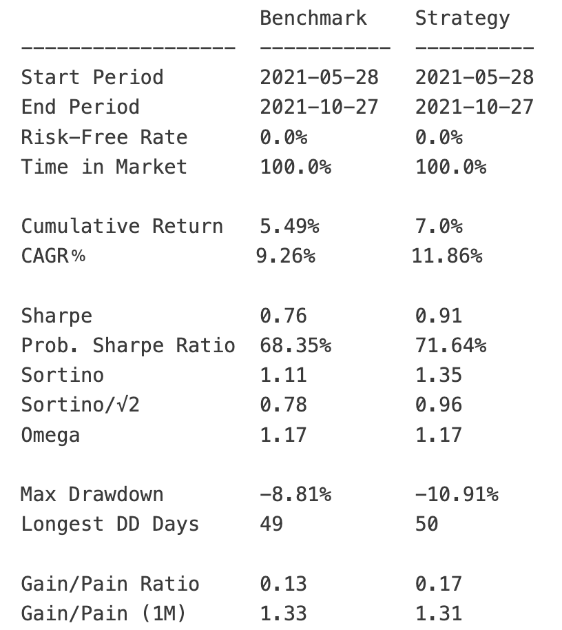
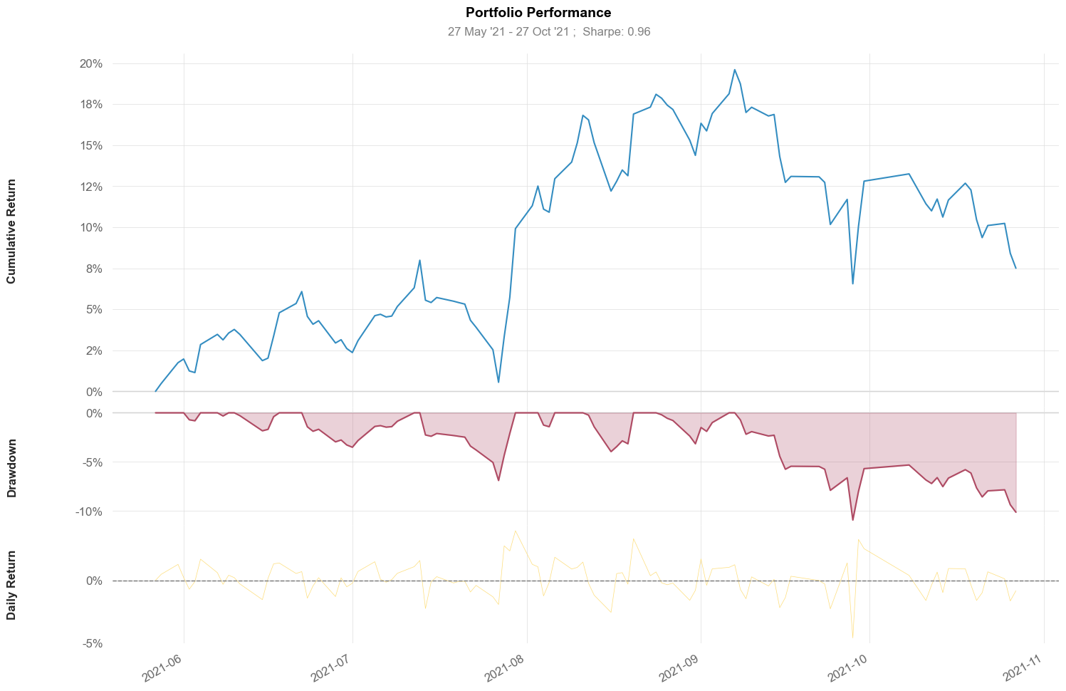
Thus, we have completely implemented an advanced RL trading model! On this basis, you only need to do well in feature engineering and data preprocessing to continuously improve and tune it!
One More Thing
Usually, introductions to RL trading models often mention FinRL. Indeed, it is a very excellent library, but it requires YFinance—unusable in mainland China since late 2021; and it also depends on Alpaca—a library for trading US stocks.
These two dependencies cause programs using FinRL to fail to run here. This is why we implemented it from scratch.
Additionally, we must say that the devil is in the details. For example, the asset set used during training can only be used for the same asset set during testing (live trading). But when handling backtests over long time spans, errors in dataset splitting can easily lead to inconsistencies between these two sets. In quantitative trading, engineering implementation ability is as important as algorithm innovation (for most people, actually application) ability.
After manually implementing this framework, I realized that most of the data preprocessing work has actually been implemented in the Alphalens library—at least in this part, Alphalens performs robustly.
If you are interested in the content and corresponding code of this article, you might consider participating in the Factor Mining and Machine Learning Strategies course. RL is a supplementary course for this class.
In summary, RL opens a door to higher-dimensional intelligence for quantitative trading. It is no longer about machines imitating humans, but about machines self-evolving and self-playing in simulated markets, ultimately acquiring trading wisdom beyond human intuition. This path is full of challenges, but also full of opportunities.
So, are you ready to let your first trading Agent begin its "evolution journey"?
- LOXM: https://www.businessinsider.com/jpmorgan-takes-ai-use-to-the-next-level-2017-8
- Reinforcement Learning in Quantitative Trading: https://dl.acm.org/doi/10.1145/3582560
- Alphastock, a momentum trading model: https://arxiv.org/abs/1908.02646