Numpy Structured Arrays for Tabular Data in Quant Finance

12345678910111213141516import numpy as np
import datetime
dtypes = [
        ("frame", "O"),
        ("code", "O"),
        ("open", "f4"),
        ("high", "f4"),
        ("low", "f4"),
        ("close", "f4")
    ]
secs = np.array (
    [
        (datetime.date (2024, 3, 18), "600000", 8.9, 9.1, 8.8, 9),
        (datetime.date (2024, 3, 19), "600000", 8.9, 9.1, 8.8, 9),
    ], dtype = dtypes
)

warning

A common mistake for beginners is initializing a Numpy Structured Array using `List[List]` instead of `List[Tuple]`. This causes Numpy to fail in mapping the correct data types, resulting in obscure errors. For example, the following initialization is incorrect:

1234secs = np.array ([
    [datetime.date (2024, 3, 18), "600000", 8.9, 9.1, 8.8, 9],
    [datetime.date (2024, 3, 19), "600000", 8.9, 9.1, 8.8, 9]
], dtype=dtypes)

This code will raise an unintelligible "Type Error: float () argument must be a string or ..."

12345678910print (f"secs 的维度是 {secs.ndim}")
print (f"secs 的 shape 是 {secs.shape}")
print (f"secs 的 size 是 {secs.size}")
print (f"secs 的 length 是 {len (secs)}")

print (f"secs [0] 的类型是 {type (secs [0])}")
print (f"secs [0] 的维度是 {secs [0].ndim}")
print (f"secs [0] 的 shape 是 {secs [0].shape}")
print (f"secs [0] 的 size 是 {secs [0].size}")
print (f"secs [0] 的 length 是 {len (secs [0])}")

1234print (secs [0]["frame"])

# 不使用列名（字段名），使用其序号也是可以的
print (secs [0][0])

1print (secs ["frame"][0])

12for (frame, code, opn, high, low, close) in secs:
    print (frame, code, opn, high, low, close)

warning

When modifying cell values, the order of indexing matters and cannot be swapped: ```python data = np.array ([("aaron", "label")], dtype=[("name", "O"), ("label", "O")]) filter = data ["name"] == "aaron"

12345new_label = "blogger"
data ["label"][filter] = new_label

# this won't change
data [filter]["label"] = new_label

12345678910111213141516171819202122232425262728293031323334353637383940414243444546474849The last line above will not take effect.
</div>
## 2. Operations
### 2.1. Comparison and Logical Operations

In the previous section on locating and searching, we encountered data comparisons, such as `arr > 1`. This compares every element in the array with `1` and returns a boolean array.

Now, we expand the comparison instructions:

| Function   | Description                                                                                         |
| ---------- | --------------------------------------------------------------------------------------------------- |
| all        | Returns `True` if all elements in the array are true. Used to check if a set of conditions holds simultaneously. |
| any        | Returns `True` if at least one element in the array is true. Used to check if at least one condition holds. |
| isclose    | Checks if elements in two arrays are approximately equal element-wise, returning all comparison results. |
| allclose   | Checks if all elements in two arrays are approximately equal.                                       |

---

| Function     | Description                                                                                       |
| ------------ | ------------------------------------------------------------------------------------------------- |
| equal        | Checks if elements in two arrays are equal element-wise, returning all comparison results.          |
| not_equal    | Checks if elements in two arrays are not equal element-wise, returning all comparison results.      |
| isfinite     | Checks if elements are finite numbers (not infinite).                                               |
| isnan        | Tests if elements are Not-a-Number (NaN).                                                           |
| isnat        | Tests if objects are not of datetime type.                                                          |
| isneginf     | Tests if objects are negative infinity.                                                             |
| isposinf     | Tests if objects are positive infinity.                                                             |


```python
# 开启多行输出模式
from IPython.core.interactiveshell import InteractiveShell
InteractiveShell.ast_node_interactivity = "all"

np.random.seed (78)
returns = np.random.normal (0, 0.03, size=4)
returns
# 判断是否全下跌
np.all (returns <= 0)
np.any (returns <= 0)

# 模拟一个起始价格为 8 元的价格序列
prices = np.cumprod (1+returns) * 8

# 对应的涨停价如下
buy_limit_prices = [8.03, 8.1, 8.1, 8.3]

# 判断是否涨停
np.isclose (prices, buy_limit_prices, atol=1e-2)

---

Therefore, if we have the closing price and the price limit (up-limit) of a stock, to determine if the stock has hit the up-limit, we must use `isclose` for comparison, not `equal`.

The parameter atol represents the absolute tolerance. If the difference between two floating-point numbers is less than this value, they are considered approximately equal.

Beyond checking if all elements in an array are True or if at least one is True, we sometimes need fuzzy judgments. For example, if more than 60% of the past 20 days showed bullish candles (positive returns), we can use np.count_nonzero or np.sum to count the True values in the array:

12np.count_nonzero (returns > 0)
np.sum (returns > 0)

In the previous comparison examples, we only used single conditions. To search based on combinations of multiple conditions, we rely on logical operations.

In Numpy, logical operations can be performed via functions or operators:

---

Function	Operator	Description	Python Equivalent
logical_and	&	Performs logical AND	and
logical_or	|	Performs logical OR	or
logical_not	~	Performs logical NOT	not
logical_xor	'^'	Performs logical XOR	xor

What is the use of logical operations? For example, in stock selection, we might have the following tabular data:

Stock	PE	MOM
AAPL	30.5	0.1
GOOG	32.3	0.3
TSLA	900.1	0.5
MSFT	35.6	0.05

The above table can be represented as a Numpy Structured Array:

123456tickers = np.array ([
    ("APPL", 30.5, 0.1),
    ("GOOG", 32.3, 0.3),
    ("TSLA", 900.1, 0.5),
    ("MSFT", 35.6, 0.05)
], dtype=[("ticker", "O"), ("pe", "f4"), ("mom", "f4")])

---

Now, suppose we want to find records where PE < 35 and Momentum (MOM) > 0.2. We can construct the condition expression as follows:

1(tickers ["pe"] < 35) & (tickers ["mom"] > 0.2)

Numpy compares all values in the PE column with 35, then performs a logical AND with the results of comparing MOM with 0.2. This is equivalent to:

1np.array ((1,1,0,0)) & np.array ((0, 1, 1, 0))

In Numpy, True is equal to 1 in logical operations, and 0 is equal to False.

Without Numpy's logical operations, we would have to use Python's logical operators, which require loops. If the computation volume is large, this would be time-consuming.

An example of using XOR in quantitative finance is stock selection. For instance, if we require that only one of two selection conditions holds before buying (otherwise, do not buy), we can use the XOR operation.

---

### 2.2. Set Operations

In trading, we often perform rebalancing operations. The general approach is to determine a new portfolio, compare it with the current portfolio, and identify stocks to sell and stocks to buy. This operation is known as set operations. In Python, this is typically implemented using set syntax.

In Numpy, we can implement set operations using the following methods:

12345678910111213141516import numpy as np

# 创建两个一维数组
x = np.array ([1, 2, 3, 4, 5])
y = np.array ([4, 5, 6, 7, 8])

# 计算交集
intersection = np.intersect1d (x, y)
print ("Intersection (交集):", intersection)

# 计算并集
union = np.union1d (x, y)
print ("Union (并集):", union)

diff = np.setdiff1d (x, y)
print ("x - y:", diff)

---

Additionally, we might use the in1d(a1, a2) method to check if all elements in a1 exist in a2. For example, in portfolio rebalancing, if the current holdings are all included in the buy plan, no rebalancing is needed.

2.3. Mathematical and Statistical Operations

Numpy supports various mathematical operations, including linear algebra (and basic algebra), statistical operations, and financial indicator calculations.

2.3.1. Linear Algebra

Linear algebra is crucial in quantitative finance. For example, in Modern Portfolio Theory (MPT), calculating portfolio returns and covariances requires matrix multiplication. You can refer to the Portfolio Theory and Practice series for more details. Below is a snippet of code:

123...
cov = np.cov (port_returns.T)
port_vol = np.sqrt (np.dot (np.dot (weights, cov), weights.T))

Matrix multiplication is a core concept in linear algebra, involving the specific multiplication and summation of elements from two matrices to generate a new matrix. Specifically, if matrix $A$ is of dimension $m \times n$ and matrix $B$ is of dimension $n \times p$, their product $C = AB$ will be a matrix of dimension $m \times p$. The rule is that each element of a row in $A$ is multiplied by the corresponding element of a column in $B$, and the results are summed.

The following example illustrates the process of matrix multiplication:

Suppose we have two matrices $A$ and $B$:

---

$$ A = \begin {bmatrix} 2 & 3 \ 1 & 4 \ \end {bmatrix} $$ and $$ B = \begin {bmatrix} 1 & 2 \ 3 & 1 \ \end {bmatrix} $$ To calculate $AB$, we follow these steps:

Take the first row of $A$ $(2, 3)$ and the first column of $B$ $(1, 3)$, multiply corresponding elements, and sum them to get $C_{11} = [2\times1 + 3\times3 = 11]$.

Similarly, take the first row of $A$ and the second column of $B$ $(2, 1)$, multiply corresponding elements, and sum them to get $C_{12} = [2\times2 + 3\times1 = 7]$.

Take the second row of $A$ $(1, 4)$ and the first column of $B$, multiply corresponding elements, and sum them to get $C_{21} = [1\times1 + 4\times3 = 13]$.

Take the second row of $A$ and the second column of $B$, multiply corresponding elements, and sum them to get $C_{22} = [1\times2 + 4\times1 = 5]$.

Therefore, matrix $C = AB$ is:

$$ C = \begin {bmatrix} 11 & 7 \ 13 & 6 \ \end {bmatrix} $$

Unlike algebraic operations, matrix multiplication is not commutative, meaning generally $AB \neq BA$.

In Numpy, we can use the np.dot() function to calculate matrix multiplication.

---

The above example expressed in numpy is:

1234A = np.array ([[2,3],[1,4]])
B = np.array ([[1,2],[3,1]])

np.dot (A, B)

Finally, we obtain the same result as matrix $C$.

Additionally, matrix inversion (np.linalg.inv) is used to solve systems of equations when calculating optimal portfolio weights. Eigenvalues and eigenvectors (np.linalg.eig, np.linalg.svd) are used in analyzing the principal components of asset returns and performing risk decomposition.

2.3.2. Statistical Operations

Common statistical operations include:

Function	Description
np.mean	Calculates the mean.
np.median	Calculates the median.
np.std	Calculates the standard deviation.
np.var	Calculates the variance.
np.min	Calculates the minimum value.
np.max	Calculates the maximum value.
np.percentile	Used to calculate percentiles of historical data.
np.quantile	Used to calculate quantiles of historical data; same function as percentile.
np.corr	Used to calculate correlation between two variables.

np.percentile and np.quantile serve the same purpose: calculating quantiles.

---

They differ slightly in parameters. When applying them to the same array, passing a quantile of 0.25 to quantile yields the same result as passing a percentile of 25 to percentile (the latter is multiplied by 100). In quantitative trading, quantile is used more frequently.

A common application of `np.percentile` (or `np.quantile`) is calculating the 25%, 50%, and 75% quantiles to draw box plots (Boxplot).

We also frequently use it to select adaptive parameters. For example, in RSI applications, it is generally recommended to buy when below 20 (or 30) as oversold, and sell when above 80 (or 70) as overbought. However, with some statistical analysis, you will find these thresholds are not fixed. If we use the RSI over a past period to find its 95% quantile as the sell point and the 15% quantile as the buy point, we often achieve better results.

2.3.3. Calculation of Quantitative Indicators

Some common quantitative indicator calculations can also be performed using Numpy. For example, calculating moving averages can be done using Numpy's convolve function.

12345import numpy as np
def moving_average (data, window_size):
    return np.convolve(data,
                       np.ones(window_size)/window_size, 
                       'valid')

---

Of course, many people are accustomed to using talib or Pandas' rolling function for calculations. convolve (convolution) is the core of neural networks (CNNs), which is why we mention it here.

The second parameter of np.convolve is the convolution kernel. Here, we are implementing a Simple Moving Average (SMA), so the convolution kernel is an array of identical values. Its length is the window size, and the sum of its elements is 1.

If we replace the convolution kernel with other values, we can implement indicators like WMA. From a signal processing perspective, moving average is a form of signal smoothing. Using different convolution kernels achieves different smoothing effects.

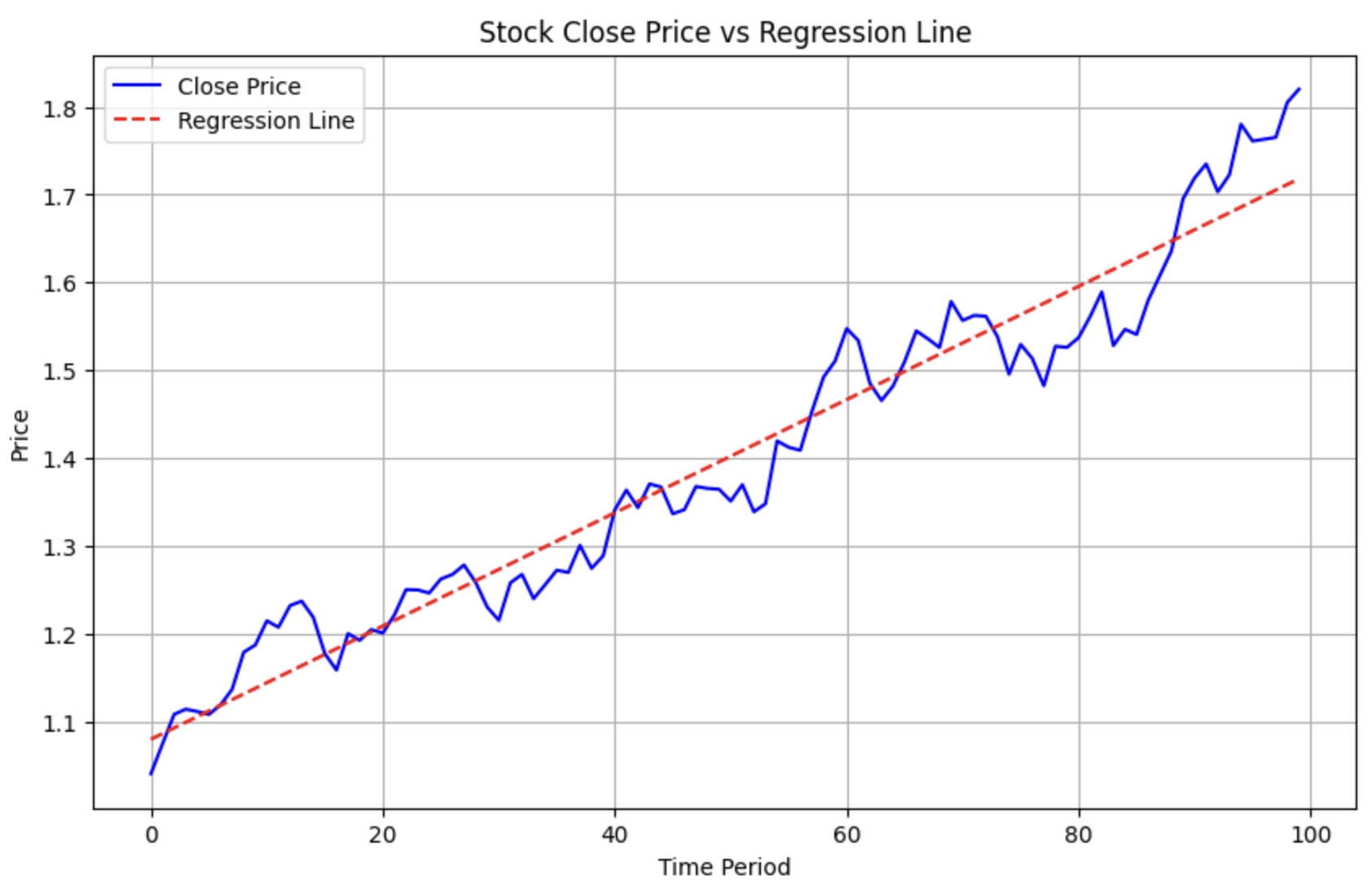
In quantitative finance, another type of calculation worth mentioning is polynomial regression. For example, if two stocks have recently shown an upward trend, and we want to know which one is performing better, we can perform polynomial regression, fit them to a line, and then compare their slopes.

The following code demonstrates how to use Numpy for polynomial regression.

1234567891011import numpy as np
import matplotlib.pyplot as plt

returns = np.random.normal (0, 0.02, size=100)
alpha = 0.01
close = np.cumprod (1 + returns + alpha)

a, b = np.polyfit (np.arange (100), close, deg=1)

# 使用 a, b 构建回归线的 y 值
regression_line = a * np.arange (100) + b

---

12345678910111213141516# 绘制原始的 close 曲线
plt.figure (figsize=(10, 6))
plt.plot (close, label='Close Price', color='blue')

# 绘制回归线
plt.plot (regression_line, label='Regression Line', color='red', linestyle='--')

# 添加图例、标题和坐标轴标签
plt.title ('Stock Close Price vs Regression Line')
plt.xlabel ('Time Period')
plt.ylabel ('Price')
plt.legend ()

# 显示图表
plt.grid (True)
plt.show ()

This will generate the following image:

---

Cover Image: Photo by Steve Harvey on Unsplash