Herd Behavior in China A-Shares and How to Factorize It

In previous notes, we've repeatedly paired modern finance theory with popular China A-shares sayings, market lore, and lessons from star influencers — we jokingly call it the Sinicization of modern finance theory. This note continues that thread, covering the herd effect: how it shows up in China A-shares, how to factorize it, and more.

The saying for today comes from Yang Jia's playbook: win over retail investors and you win the world. It is really about exploiting the herd effect to the fullest.

Herd effect theory, also known as herd behavior or herding instinct, is a key pillar of behavioral finance.

Economists often use "herd effect" to describe the follow-the-crowd psychology of economic agents. A sheep flock is a loose organization: once the lead sheep moves, the rest follow, never stopping to ask whether a wolf lies ahead (danger), or whether they are walking away from lush pasture (reward).

In investing, the herd effect is at work almost all the time. Even in value investing it is strikingly obvious. People will pay millions for a lunch with Warren Buffett just to get a few investment tips. The most famous Buffett episode in China A-shares was his purchase and endorsement of a certain oil giant, which triggered a wave of retail copycats who ended up trapped at the top near 6,000 points.

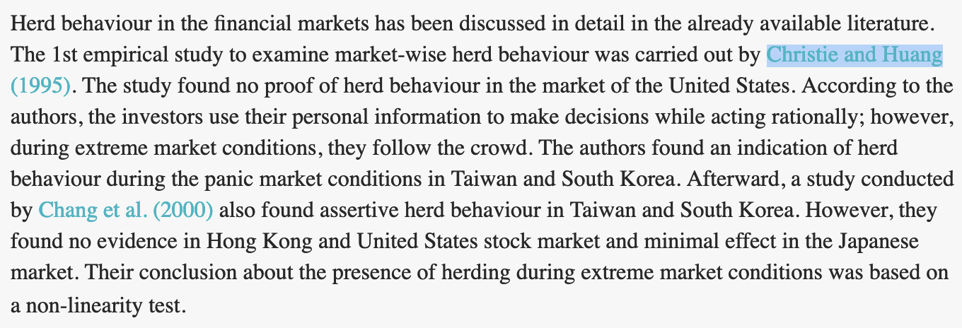
In 1995, Christie and Huang published the first empirical study of market-wide herd behavior. They found no evidence of herding in the US, Japanese, and Hong Kong markets, but found fairly conclusive evidence in Taiwan and South Korea.

As a quant blogger, I care more about how to turn this effect into factors. Here are a few related ones.

New Account Openings Factor

Monthly new account openings can be fetched via AKShare:

12345import akshare as ak

# 得到每月新开户人数
accounts_df = ak.stock_account_statistics_em()
accounts_df

This gives us investor account data going back to April 2015.

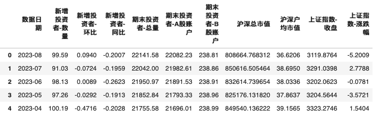
In the returned table, one column holds the data date in a format like "2015-04", which we need to convert into a proper date format.

123456# 这里演示了如何取 DATAFRAME 的数据单元
end = accounts_df.iloc[0]["数据日期"]
start = accounts_df.iloc[-1]["数据日期"]

yr, month = end.split("-")
end = datetime.date(int(yr), int(month) + 1, 1)

1234567# tf.floor 是 OMICRON 的函数，它将日期对齐到上一个已结束的周期
# 在 OMICRON 中，提供了大量时间运算函数，是量化中必备的
end = tf.floor(end, FrameType.MONTH)

yr, month = start.split("-")
start = datetime.date(int(yr), int(month) + 1, 1)
start = tf.floor(start, FrameType.MONTH)

We now have the start and end dates from the investor account data, so we can pull index prices and plot them together.

1234567891011121314
# 获取上证指数
bars = await Stock.get_bars_in_range("000001.XSHG", 
                                    FrameType.MONTH, 
                                    start, end)

# 将新增投资者人数与上证指数走势对应起来
df = pd.DataFrame({"xshg": bars["close"][::-1] / 10, 
                   "investor": accounts_df["新增投资者-数量"]})
df.index = accounts_df["数据日期"]

fig = px.line(df)
fig.update_layout(hovermode="x unified")
fig.show()

The relationship looks like this:

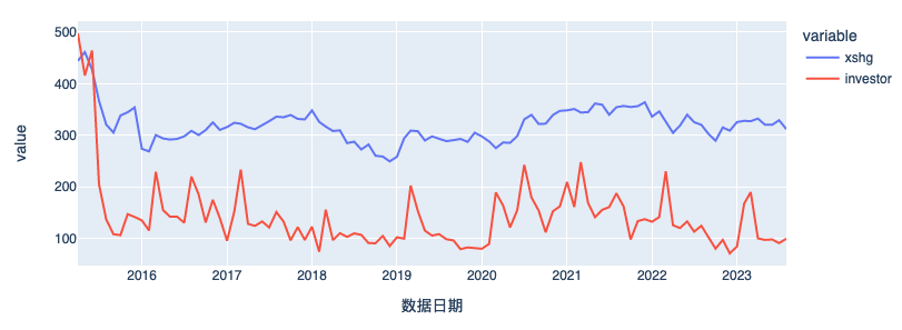
You can see that monthly new investors fluctuate within a band of roughly 1 million at the low end to 2.2 million at the high end. This band correlates to some extent with what the Shanghai Composite does next. By eyeballing it: when new openings sit near the lower bound, the index is near a bottom about 70% of the time; when they sit near the upper bound, the index is near a top about 70% of the time.

That is just a visual pattern. In Part 3 of the course (Statistical Science and Python Data Analysis), we'll show how to describe this kind of correlation with proper statistics. After Part 3, we'll also know how to answer: if new openings hit 2 million this month, what is the probability they keep rising next month?

That matters a lot. After all, in a game of musical chairs, the drumbeat must not stop.

Popularity Ranking Factor

AKShare offers a function that pulls the Guba forum popularity ranking for a given ticker. The popularity ranking is clearly a classic retail-investor gauge — institutions have the money, retail investors have the headcount.

The usage is:

123import akshare

akshare.stock_hot_rank_detail_realtime_em("SZ000665")

The output looks like this:

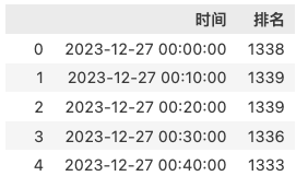
The data here is rich enough. Whether it can work as a factor is something you can test with Alphalens.

Conclusion

China A-shares is a market with a pronounced herd effect — win over retail investors and you win the world. Here I've shown just two factor examples; many more remain to be discovered.

As a quant-framework developer, I strongly believe in learning from star retail traders and top influencers. In future notes I will keep unpacking the modern finance theory behind their playbooks and try to quantify it.

I've set up a Xiaohongshu study check-in group — feel free to join if you want to keep learning together. Today's check-in quote: