Max Volume Factor: Mining Alpha via Smart Money Footprints

Because of the night, we can see the starry sky more clearly | ©️ Nathan Jennings

I recently chatted with a friend who wants to transition into the quantitative finance industry. He was worried it might be too late or that the macro environment wasn’t favorable. So, I encouraged him with this quote:

Because of the night, we can see the starry sky more clearly.

In the depths of a downturn, there is always a turning point; after enduring the darkness, light awaits ahead.

In fact, several "ordinary" people around me have successfully pivoted to quantitative investing. A former strategy researcher recently called me to share that a private equity firm had approached him to purchase his strategy. He has even registered his own company. He is a true legend, and I will share his story at the appropriate time to inspire others.

Do what you love, ignore the labels others place on you, and don’t let others define you.

You gotta be brave.

As long as you are willing to chase your dreams, you are not mediocre.

Now, back to business.

In Lesson 12, I promised to discuss how to discover new factors. Words alone are not enough; I must deliver a factor (strategy) that has not yet been widely disseminated. Today, I fulfill that promise. When exploring factors, we generally look at four dimensions: volume, price, time, and space. Among these, volume-based factors are the least explored. Therefore, today I will introduce a factor I discovered myself.

If there are similarities, it’s purely a coincidence (due to limited reading). This factor is based on trading volume and constructed using the principle of herd behavior.

Have All Factors Been Mined?

Before diving into the details, let’s answer a question: Have all factors been mined? After all, there are so many quantitative researchers worldwide.

The fact is that global computational power is insufficient, meaning many relationships remain undiscovered. The story of Rolf Banz, the father of the small-cap factor, illustrates this point well.

Around 1980, Rolf Banz published the paper The relationship between return and market value of common stocks, introducing the small-cap factor to the world.

Banz’s paper is not complex, spanning only 16 pages. It does not use advanced mathematics but relies on basic statistical science, specifically GLS and OLS. If computers were available at the time, the derivation process would appear remarkably simple.

In fact, we can understand the small-cap factor solely from the chart in his paper:

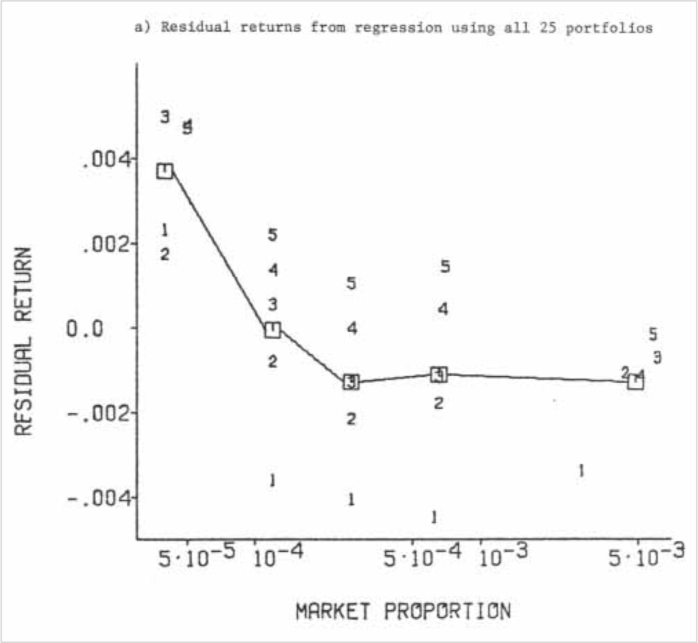Relationship between Returns and Market Cap Deciles

In this chart, Banz grouped assets into five buckets by market capitalization. Group 1 represents the smallest market cap, and Group 5 represents the largest. Clearly, the returns of the other groups have a linear relationship with market cap, but Group 1 (small-cap) exhibits higher monthly returns that cannot be explained by linear regression.

This simple fact earned Banz the title of "Father of Small-Cap." If William Sharpe discovered the first factor, Banz discovered the second.

The data Banz used came from 1926 to 1975, stored in the CRSP database at the University of Chicago. For over 50 years, it quietly waited for someone to uncover its value. The University of Chicago has produced numerous economics talents, and countless people may have accessed this data. Yet, Banz was the one to pluck this low-hanging, aromatic fruit.

I believe this sufficiently demonstrates that in any era and any circle, there are always low-hanging fruits waiting for the diligent to pluck them.

However, even more astonishing is that another low-hanging fruit appeared in Banz’s own paper. In the chart above, assets were actually divided into 25 groups. Within each market-cap bucket, Banz further subdivided assets by volatility into five groups (vertically distributed in the chart). Group 1 represents the highest volatility, and Group 5 represents the lowest.

Clearly, within every combination, assets with low volatility yielded higher returns than those with high volatility.

In fact, another factor emerged here: the low-volatility factor. Our backtests show that a daily low-volatility factor can achieve an annualized Alpha of 16.4%, while a monthly version achieves around 6.3%, with a Factor IC of 0.04, which is quite substantial.

Then, ten years later, Haugen and Baker discovered and named the low-volatility factor. Banz had done almost all the work but missed this invention.

Low-hanging fruits will always exist

The Max Volume Factor

This factor can also be called the "Smart Money Factor." Its construction principle is that price direction is determined by smart money. When individuals are part of a group, their behavior and decisions are influenced by the crowd, often leading to a loss of rationality and increased emotionalism and impulsiveness. Individuals tend to be guided by others and ultimately follow the direction of the lead sheep—this is herd behavior.

Only smart money can determine the direction; the force determining the direction is smart money. Therefore, the direction of smart money can be modeled.

123456789101112131415161718192021222324252627282930import pandas as pd

def max_volume_direction(df, win=40):
    old_index = df.index.copy()
    df = df.reset_index().set_index(np.arange(len(df)))
    df["flag"] = np.select([
        df["close"] > df["open"],
        df["close"] < df["open"]
    ], [1, -1], 0)

    df["move_vol_avg"] = df["volume"].rolling(window=win, min_periods=win).mean().shift(1)
    df["argmax"] = df['volume'].rolling(win, min_periods=win).apply(lambda x: x.idxmax())
    df.fillna(0, inplace=True)
    df["move_vol_max"] = df.apply(lambda row: df.loc[row['argmax'], 'volume'], axis=1)
    df['vr'] = df['volume'] / df['move_vol_avg'] * df["flag"]
    df["span"] = df.index - df["argmax"]

    def calc_rolling_net_balance(df):
        pos = df["argmax"].iloc[-1] + 1
        sub = df.loc[pos:,]
        return (sub["flag"] * sub["volume"]).sum() / df["move_vol_max"].iloc[-1]

    balances = []
    for sub in df.rolling(win):
        b = calc_rolling_net_balance(sub)
        balances.append(b)

    df["move_balance"] = balances

    return df[["vr", "move_balance", "span"]].set_index(old_index)

The logic of this code is as follows: if a bar’s trading volume is abnormally high relative to the average volume over a recent period (calculated as the bar’s volume divided by the average volume, denoted as vr), it may indicate smart money activity. We assume that the direction of this bar is highly likely to be the subsequent direction of smart money operations.

If this bar is a bullish candle (yang line), it reflects buying activity; if it is a bearish candle (yin line), it reflects selling activity (denoted as flag).

To test counter-parties and follow-on traders, smart money may pause operations after a trial run to observe market changes. Therefore, we examine trading conditions for a period after this bar, converting this volume into net residual volume (denoted as move_balance), and then normalizing it by dividing by the volume of the smart money bar. If the net residual volume is in the same direction as the smart money bar, it indicates minimal counter-pressure (or no intent to counter); if the net residual volume is significantly opposite to the smart money bar, the smart money’s intent may be difficult to achieve, and they may temporarily abandon the operation.

Let’s test this with a sample:

123456789101112131415161718192021222324252627import akshare as ak
def test(bars, thresh=5):
    bars.index = np.arange(len(bars))
    df = max_volume_direction(bars, 40)

    bars.rename(columns={"day": "date"}, inplace=True)
    cs = Candlestick(bars, height=750)
    # add up markers
    df["close"] = bars["close"]
    x = df[np.isfinite(df.vr) & (df.vr > thresh)].index
    y = df[np.isfinite(df.vr) & (df.vr > thresh)]["close"] * 1.05
    cs.add_marks(x, y, name="up", marker="triangle-up")

    # add down markers
    x = df[np.isfinite(df.vr) & (df.vr < -thresh)].index
    y = df[np.isfinite(df.vr) & (df.vr < -thresh)]["close"] * 0.95
    cs.add_marks(x, y, name="down", marker="triangle-down", color="green")

    cs.plot()

code = "sz002466"
bars = ak.stock_zh_a_minute(symbol=code, period="30", adjust="qfq")
bars = bars[-150:].copy()

bars["volume"] = bars.volume.astype(int)

test(bars)

In the test, we set the threshold for vr to 5. For more aggressive individual stocks, setting it above 8 may yield better results.

In the example, we see three upward arrows. After the first two appeared, the stock price subsequently fell, but the opposite volume was minimal, indicating no counter-selling pressure. Thus, smart money later pushed the price up again. After the third arrow appeared, significant selling pressure signals (doji/star patterns) emerged, and the stock price subsequently fell.

Of course, we still need to conduct large-scale testing. These are the topics covered in Factor Analysis and Machine Learning Strategies. Regarding factor innovation, we have provided innovative ideas and directions across the four dimensions of volume, price, time, and space. Stay tuned for continuous updates!