
PDF Is All You Need (3): From Galton Board to Expected Value
In the previous installment, we introduced the binomial distribution and noted:
Probability of exactly k events in a binomial distribution
$$ P(X=k) = C_{(n,k)} \times p^k \times (1-p)^{n-k} $$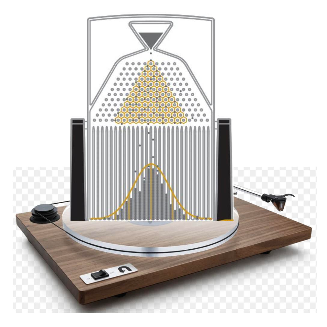 Figure 1: Galton Board
info
The Galton Board was designed by British scientist Francis Galton, a cousin of Charles Darwin. He proved that fingerprints are unique and stable throughout a person's life. He also coined the term "eugenics," which remains highly controversial today.When we drop a ball from the entry, it hits the nails in the middle and bounces either left or right until it hits the next nail or falls into one of the vertical dividers at the bottom. By calculating the ratio of the number of balls in each slot to the total number of balls, we can determine the probability of choosing "right" or "left" $k$ times out of $n$ collisions.
In essence, the lower half of the Galton Board corresponds to the histograms commonly used in statistics. The width of the slots can be viewed as the "bin width," while the height of the ball accumulation (slot height) corresponds to the "frequency." However, when drawing histograms, we can arbitrarily specify the bin width.
What happens if we increase the number of nails and the number of trials in such a device? The figure below shows a possible outcome with 20 layers of nails and 500 trials:
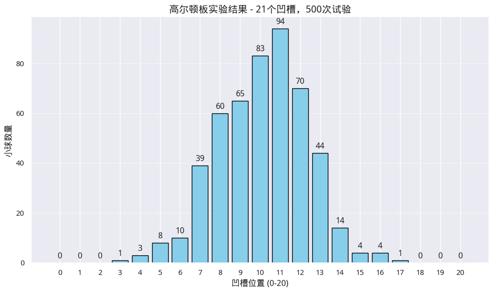 Figure 2: Result after hitting nails 10,000 times!
tip
To simulate this experiment, we need to use the `binomial` function from `numpy.random`. It efficiently simulates a series of independent Bernoulli trials.</div>
from numpy.random import binomial, histogram
right_turns = binomial(n=layers, p=0.5, size=balls)
counts, _ = histogram(right_turns, bins=np.arange(layers + 2))在这个图中,如果我们把每一个凹槽按位置进行编号,把小球落入的位置看成事件的取值,那么我们就得到了一个离散型的随机变量。在图2中,它的取值区间是[0, 20]。
如果我们增加层数,多试验几次,又会如何?下图显示了1000个凹槽、1百万次试验的一种可能结果:
 图3 频率/随机变量图
我们看到随机变量的中心值是500左右 -- 说明我们的实验是正确的,因为凹槽的个数是1000。但最小值与最大值并不是0和1000,这是因为我们试验的次数还不够多,要使得二项分布取到这样的极限值还是非常困难的。但是,如果凹槽的个数只有10个,而试验次数达到1000次,就很容易取到(0, 10)这两个极值了。
或许你已经注意到,这次的图跟图2有一点不一样。这次我们绘制的实际上不再是直方图,而是概率密度/随机变量图。我们用来绘制这张图的代码是:
import matplotlib.pyplot as plt
plt.hist(positions, bins=num_grooves, density=True)The key parameter here is density=True. When specified as True, the hist plotting function’s y-axis no longer represents the frequency of each bin but the probability density.
How is this probability density calculated? In Figure 3, we divide random numbers falling roughly within the range (428, 575) into 1,000 average bins, resulting in 1,000 bins with a width of approximately 0.147. Let $X_i$ be the number of random numbers (balls) falling into each bin. Then, $\frac{X_i}{n \times 0.147}$ is the probability density of $X$ in that bin. Geometrically, multiplying this probability density by the bin length (i.e., the area of the small rectangle) yields the probability of the ball falling into that interval.
Sum of all rectangle areas
Now, consider this question: if we calculate the area of these 1,000 rectangles and sum them up, what will we get?If we further increase the number of slots and trials—for example, increasing the slots to 10,000—what happens? Eventually, each bin and its corresponding probability density will be so tightly packed that they become visually indistinguishable, yielding the following figure:
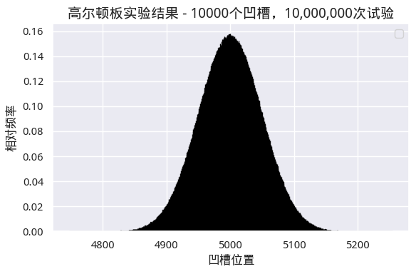 Figure 4: Approaching a Normal Distribution
However, this figure is still composed of several rectangles. For any $X_i$, we can calculate the probability of $X \ge X_i$ by summing the areas of the first $i$ rectangles. Although the number of rectangles increases, the sum of the areas of all small rectangles remains 1.
What if we continue to increase the number of nail layers and trials, letting them approach $+\infty$? At this point, not only do the rectangles disappear from the screen, but they also cease to physically constitute rectangles. Instead, we see a smooth, bell-shaped curve.
What happens during this approach to infinity? In the Galton Board, the possible values of the random variable (the slots where the ball can land) are finite and discrete. However, as $n$ and the number of nail layers (which correspond to the number of slots) approach infinity, the possible values of the random variable transition from discrete to continuous.
Now, to calculate the probability of the event $X \ge X_i$, we can no longer use the sum of small rectangle areas. However, as the length of the small rectangles approaches zero, the summation becomes the definition of an integral. Thus, we obtain the distribution function expressed via integration.
PDF and CDF
In the previous discussion, we have encountered the PDF (Probability Density Function) and CDF (Cumulative Distribution Function). The former is translated as the probability density function, and the latter as the cumulative distribution function, often simply referred to as the distribution function.
tip
We can now perhaps understand the meaning of the `density` parameter in the `plt.hist` method. It indicates that we require the y-axis values to represent probability density, not frequency.$$ F(x) = P(X\le x) = \int_{-\infty}^{x} f(t) dt \tag {CDF} $$
$$ f(x) = F'(x) \tag {PDF} $$
$$ P(X_a \leq x < X_b) = \int_{a}^{b} f(t) dt \tag {Probability of X falling between a and b} $$
Therefore, the PDF is the first derivative of the CDF, reflecting the rate of change of the CDF at a given point. The CDF represents the probability that the random variable takes a value less than or equal to $x$.
To understand the calculation of the CDF and PDF, let’s take a simple example: the probability density function of a uniform distribution.
Assume random variable $X$ is uniformly distributed over the interval $[0,n]$. The probability density is $f(x) = \frac{1}{n}$, and the probability distribution function is $F(x) = \frac{x}{n}$.
At this point, the probability that random variable $X$ falls within the interval $[a,b]$ ($0<a<b<n$) is:
$$ \begin{align} \int_a^b\frac{1}{n}dx = \frac{b-a}{n} \end{align} $$
To help everyone understand, here is an example from a quantitative finance context, which was discussed in detail in "Quantitative Trading 24 Lessons."
Given that the Shanghai Composite Index has dropped by 4% on a given day, what is the probability of success if we buy the dip now?
We can treat the daily return of the Shanghai Composite Index as a random variable. Assume we know its probability density function is $f(x)$. If the index has already dropped by 4%, the probability of further dropping is the probability that the random variable takes a value less than or equal to $x$ (currently -0.04), which is: $$p = \int_{-\infty}^{-0.04} f(x) dx$$ Given the probability of further dropping is $p$, then $1-p$ is the probability of successfully buying the dip.Expected Value
After the previous installment of "PDF Is All You Need" was published, some readers asked if we could discuss gambling probabilities (roughly speaking). I’m not very familiar with these terms, but it seems to be related to expected value.
In gambling, Expected Value is the core tool for analyzing strategy selection and evaluating the优劣 (pros and cons) of situations, especially in scenarios involving uncertainty (such as opponent strategies or random outcomes). Its core logic is: by calculating the expected returns (or losses) of different strategies, choose the optimal strategy that maximizes one’s own benefits (or minimizes risk).
Expected Value (also known as the mean) is the weighted average of the values taken by a random variable, where the weights are the probabilities corresponding to each value.
Expected value is generally denoted by the symbol $E(x)$, where $X$ is the random variable. If $X$ is discrete, the expected value is the sum of "the value of each outcome × the probability of that outcome occurring," i.e.:
$$ E_x = \sum_{i}^{n}X_{i}.P_i $$
Here, $X_i$ is the $i$-th outcome, and $P_i$ is the corresponding probability.
For continuous cases, calculating the expected value is somewhat more complex. Since there is no corresponding probability for $X_i$, only a corresponding probability density, the expected value must be calculated via integration:
$$ E(X) = \int_{-\infty}^{+\infty} x \cdot f(x) , dx $$
It can be understood as the "weighted area" formed by the probability density function (PDF) curve and the coordinate axes. Essentially, it is equivalent to calculating the centroid of a special shape.
We can use the following code to plot both the "weighted area" and the "center of gravity."
import numpy as np
import matplotlib.pyplot as plt
from scipy.stats import norm
# 定义正态分布:均值=5,标准差=1
mu, sigma = 5, 1
# 定义 X,pdf, x·f(x)
x_norm = np.linspace(mu-3*sigma, mu+3*sigma, 1000)
y_norm_pdf = norm.pdf(x_norm, mu, sigma)
y_norm_g = x_norm * y_norm_pdf
mask = x_norm <= 6
plt.figure(figsize=(10, 8))
# 第一个子图:正态分布的PDF
plt.subplot(2, 1, 1)
plt.plot(x_norm, y_norm_pdf, 'b-', label=f'正态分布 N({mu}, {sigma}^2) 的PDF')
# 只填充到x=6的区域
plt.fill_between(x_norm[mask], y_norm_pdf[mask], alpha=0.3, color='blue')
# 计算第一个子图中到x=6的积分值(累积概率)
integral_pdf_up_to_6 = np.trapezoid(y_norm_pdf[mask], x_norm[mask])
# 计算子图1中,到 X=6 时的重心
area = np.trapezoid(y_norm_g[mask], x_norm[mask])
centroid = area / integral_pdf_up_to_6
# 标注积分值
plt.annotate(f'x=6时的累积概率: {integral_pdf_up_to_6:.2f}',
xy=(6, 0),
xytext=(6-1.5, 0.3),
arrowprops=dict(facecolor='black', shrink=0.05),
fontsize=10,
bbox=dict(facecolor='white', alpha=0.8))
# 绘制x=6的竖线
plt.axvline(6, color='purple', linestyle='--', label=f'x=6')
E = np.trapezoid(y_norm_g, x_norm)
plt.axvline(E, color='green', linestyle='-', label=f'期望= {E:.2f}')
plt.title('正态分布的PDF与到x=6的累积概率')
plt.legend()
plt.grid(alpha=0.3)
# 绘制 X < 6的图形的重心
plt.axvline(centroid, color='orange', linestyle='--', label=f'重心= {centroid:.2f}')
plt.annotate(f'x=6时的重心: {centroid:.2f}',
xy=(centroid, 0),
xytext=(centroid-2, 0.2),
arrowprops=dict(facecolor='black', shrink=0.05),
fontsize=10,
bbox=dict(facecolor='white', alpha=0.8))
# 第二个子图:g(x) = x·f(x)
plt.subplot(2, 1, 2)
plt.plot(x_norm, y_norm_g, 'r-', label='g(x) = x·f(x)')
# 只填充到x=6的区域
plt.fill_between(x_norm[mask], y_norm_g[mask], alpha=0.3, color='red')
# 计算第二个子图中到x=6的积分值
integral_g_up_to_6 = np.trapezoid(y_norm_g[mask], x_norm[mask])
# 标注积分值
plt.annotate(f'x=6时的积分值: {integral_g_up_to_6:.2f}',
xy=(6, 0),
xytext=(6-1, 0.3),
arrowprops=dict(facecolor='black', shrink=0.05),
fontsize=10,
bbox=dict(facecolor='white', alpha=0.8))
# 绘制x=6的竖线
plt.axvline(6, color='purple', linestyle='--', label=f'x=6')
plt.axvline(mu, color='green', linestyle='-', label=f'期望 μ = {mu}')
plt.title('正态分布的加权函数 g(x) 与到x=6的积分')
plt.legend()
plt.grid(alpha=0.3)
plt.tight_layout()
plt.show()
# 打印结果
print(f"第一个子图(PDF)到x=6的积分值(累积概率) = {integral_pdf_up_to_6:.4f}")
print(f"第二个子图(g(x))到x=6的积分值 = {integral_g_up_to_6:.4f}")
print(f"g(x) 下的总面积(期望) = {np.trapz(y_norm_g, x_norm):.2f}(理论值为 {mu})")# 因为篇幅原因,仅保留关键语句。学员可得完整 notebook
mu, sigma = 5, 1
# 定义 X,pdf, x·f(x)
x_norm = np.linspace(mu-3*sigma, mu+3*sigma, 1000)
y_norm_pdf = norm.pdf(x_norm, mu, sigma)
y_norm_g = x_norm * y_norm_pdf
mask = x_norm <= 6
plt.plot(x_norm, y_norm_pdf, 'b-', label=f'正态分布PDF')
# 计算第一个子图中到x=6的积分值(累积概率)
integral_pdf_up_to_6 = np.trapezoid(y_norm_pdf[mask], x_norm[mask])
# 计算期望
E = np.trapezoid(y_norm_g, x_norm)
plt.axvline(E, color='green', linestyle='-', label=f'期望= {E:.2f}')
# 计算子图1中,到 X=6 时的重心
area = np.trapezoid(y_norm_g[mask], x_norm[mask])
centroid = area / integral_pdf_up_to_6
plt.plot(x_norm, y_norm_g, 'r-', label='g(x) = x·f(x)')
# 只填充到x=6的区域
plt.fill_between(x_norm[mask], y_norm_g[mask], alpha=0.3, color='red')
# 计算第二个子图中到x=6的积分值
integral_g_up_to_6 = np.trapezoid(y_norm_g[mask], x_norm[mask])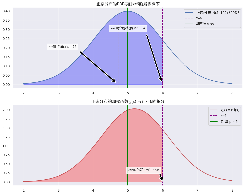 Figure 5: Normal Distribution and Expected Value
The first subplot is the density function plot of the normal distribution. Its integral is the distribution function. When $x=6$, $P(X\leq x)=0.84$. The theoretical expected value is 5, and the actual calculated value (line 14 of the code) is 4.99.
If we interpret the normal distribution density function plot as a balance scale, the position of $\mu$ is exactly in the center of the scale. This is the origin of the statement that the expected value is the center of gravity of the distribution.
The second subplot is the integral of $g(x) = x.f(x)$. When $x = 6$, the integral of $g(x)$ is 3.96. The corresponding integral of the distribution is 0.84. Therefore, the center of gravity of $g(x)$ is $3.96/0.84 = 4.72$.
tip
The expected value formula for random variable $X$ when $X \le t$ (called truncated expected value) is:$$ E(X|X\leq t) = \frac{\int_{-\infty}^{t} x f(x) dx}{\int_{-\infty}^{t} f(x) dx} $$
If you still find the integral algorithm for expected value difficult to understand after reading all this, you can try treating $x$ or $f(x)$ as a constant. Constants can be extracted from outside the integral, simplifying it to a basic integral—an object with a more intuitive physical meaning.
'Higher-Order' Expected Value
In the expected value formulas introduced earlier, we calculated the expected value of random variable $X$:
$$ E(X) = \int_{-\infty}^{\infty} x f(x) dx \tag {Eq. 1} $$
You might ask: why is the first $x$ in the equation so special? What if it is itself a function? What is the meaning of the equation:
$$ E(g(x)) = \int_{-\infty}^{\infty} g(x) f(x) dx \tag {Eq. 2} $$
First, if $g(x) = x$, then equation (2) degenerates into equation (1), i.e., both are calculating the expected value of random variable $X$. If $g(x) = 1$, then equation (2) becomes the distribution function.
Generally, whenever we see a function multiplied by a probability density and then integrated, it represents the expected value of that function. This is the meaning of equation (2).
What is the significance of this generalization? We know that discrete random variables do not have a PDF. However, if a discrete random variable $g(x)$ itself is a piecewise function, and there exists a probability density function within each piecewise interval?
At this point, equation (2) is essentially a weighted average of the function $g(X)$ of the random variable, where the weights are determined by the probability density $f(x)$ of $X$. It becomes the natural generalization of discrete expected value to continuous scenarios and is a fundamental tool for calculating the average value of functions of continuous random variables.
tip
If $g(x)$ is a piecewise, constant-type function (taking values $X_1, X_2, ...X_i$), and the integral of $f(x)$ on each segment can be denoted as $P_i$, then $\int_{1}^{i} g(x) f(x) dx = \sum_1^iX_i \cdot P_i$. As long as we see a function multiplied by a probability density and then integrated, it represents the expected value of that function.With this knowledge铺垫 (foundation), let’s return to the question posed in the first article of this series:
question
What is the probability that n randomly chosen points in a circle all lie on the same semicircle?$$ P_n = P(X_n|P_{n-1}) \times P_{n-1} \tag{3} $$
$$ \begin{align} P(X_n|P_{n-1}) &= \int P(X_n|{\alpha_{n-1}}=x) f_{\alpha_{n-1}}(x)dx \ &= \int_0^{2\pi} \frac{2\pi-x}{2\pi} f_{\alpha_{n-1}}(x) dx \end{align} \tag{4} $$
Here, $P_n$ represents the probability that $n$ randomly placed points all fall within the same semicircle. Similarly, $P_{n-1}$ is the probability that $n-1$ points all fall within the same semicircle.
$X_n$ is the event indicating that the $n$-th point and the previous $n-1$ points all lie in the same semicircle.
$P(X_n|P_{n-1})$ represents the probability that the $n$-th point also falls in the same semicircle, given that the previous $n-1$ points have already fallen in the same semicircle.
$\alpha_{n-1}$ represents the maximum angle subtended by the previous $n-1$ points when they lie in the same semicircle (i.e., the central angle between the two outermost points among these $n-1$ points, with a value range of $(0, 2\pi)$). It is also a random variable.
$f_{\alpha_{n-1}}(