Beyond Out-of-Sample: Advanced Overfitting Detection for Quant Strategies

I came across a humorous post on Zhihu describing how some strategy sellers manipulate backtest results to look better by implanting numerous if statements in their code. These checks prevent trading on specific dates, but the "secret" lies in those dates: trades on those days were all losing.

While the authenticity of this claim is questionable, it serves as a classic example of overfitting.

Overfitting and Detection Methods

Overfitting occurs when a model fits the data so closely that it fails to generalize, rendering it ineffective on new datasets. From a trading perspective, overfitting involves "designing" a strategy that performs well on historical data but will inevitably fail on new data.

Overfitting is the number one enemy in backtesting. How do we detect it?

An obvious detection method is out-of-sample testing. This involves splitting the entire dataset into non-overlapping training and test sets. The model is trained on the training set and validated on the test set. If the model performs well on the test set, we consider it not overfitted.

However, when the dataset is small, out-of-sample testing becomes difficult. To address this, extended versions have been developed.

One such extension is k-fold cross-validation, a common concept in machine learning.

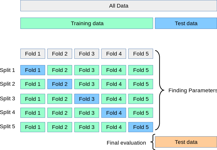
This method randomly splits the dataset into $K$ subsets of roughly equal size. For each iteration, one subset is selected as the validation set, while the remaining $K-1$ subsets form the training set. The model is trained on the training set and evaluated on the validation set. This process repeats $K$ times, and the final evaluation metric is typically the average of the $K$ validation results.

This process can be simply illustrated in the figure below:

However, in time series analysis (a typical subset of securities analysis), k-fold is unsuitable because time series data has a strict sequential order. Therefore, a specialized version derived from k-fold cross-validation is called rolling forecasting. You can view it as the sequential version of k-fold cross-validation.

It can be simply illustrated in the figure below:

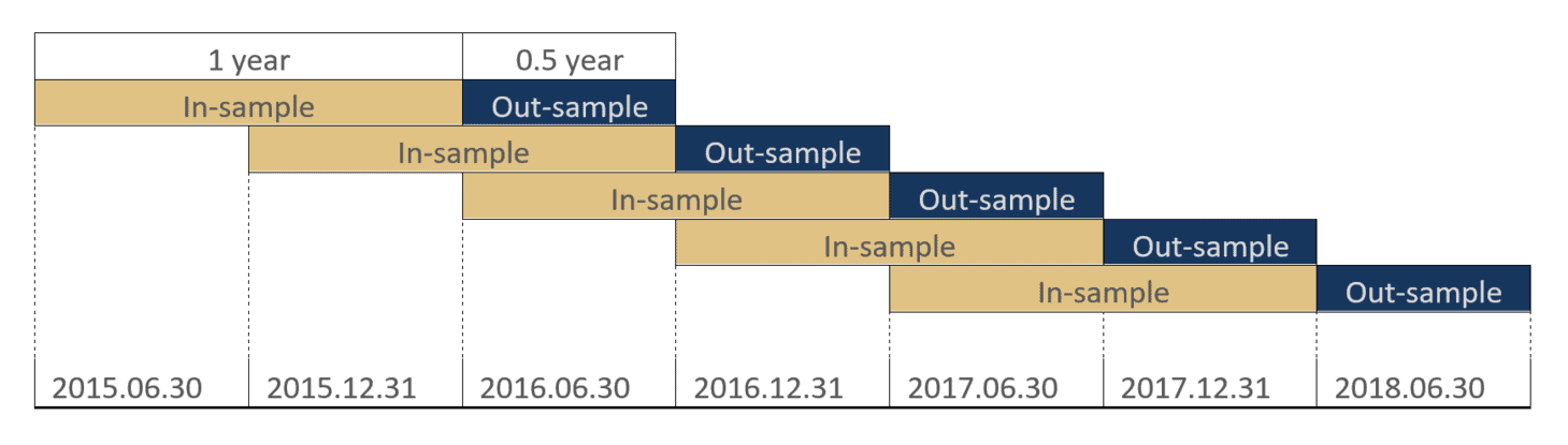
Comparing the two diagrams from k-fold cross-validation to rolling forecasting, the key difference is that one is unordered, while the other emphasizes temporal order, requiring the training and validation sets to be continuous.

You may also encounter the term Walk-Forward Optimization. It is essentially the same as rolling forecasting.

Recently, however, I learned about a novel method from the BuildAlpha website: Noise Testing.

New Attempt: Noise Testing

BuildAlpha’s noise testing involves adding a certain ratio of random noise to the backtest data, running the backtest, and then comparing the noise-based backtest results with those based on real data.

The principle is that during backtesting, historical data represents only one possible path. If time were to replay, history might not change its overall direction, but randomness would alter its steps. A robust strategy should be able to withstand randomness while capturing the overall historical trend. Therefore, adding clever noise to a time series may cause overfitted strategies to fail, while truly effective strategies will still shine.

BuildAlpha is a platform similar to TradingView. To perform noise testing, you can configure it via the graphical interface.

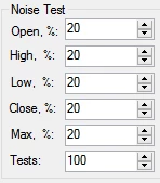
Through this dialog box, BuildAlpha modified approximately 20% of the data, keeping the modification amplitude for OHLC (Open, High, Low, Close) within 20% of the ATR (Average True Range). The "100" at the bottom indicates that 100 groups of random noisy data will be generated.

Let’s compare the real data with the noise-added data.

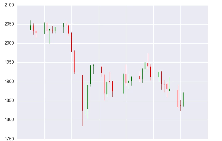
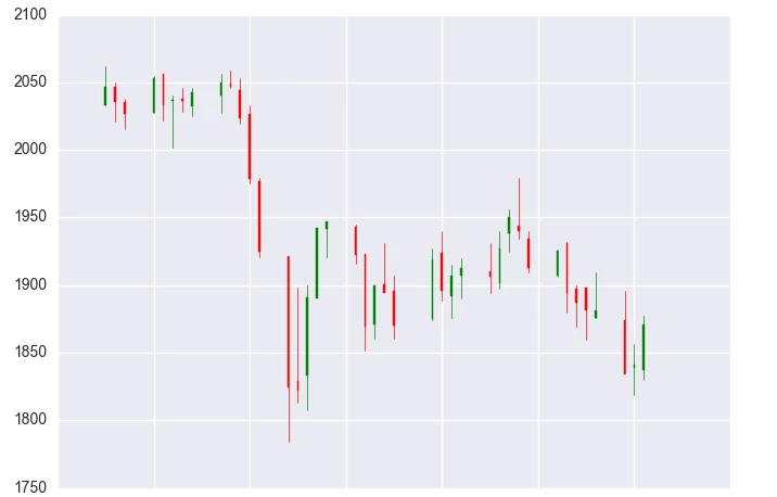
The left image shows real data, while the right shows data with added noise. The addition of noise introduces randomness in details but does not change the stock price trend (the addition is independent). If the trend were changed, this method would be invalid or even harmful.

Finally, comparing the backtest results for the same strategy yields:

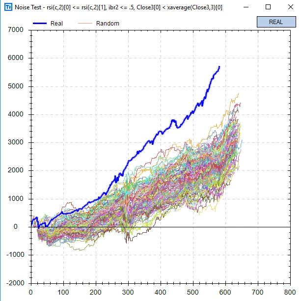
From the results, none of the multiple possible historical paths yielded better backtest results than the real data. In other words, the reason the real backtest results were so good is purely because the strategy designer had a "God’s eye view," traveling back from the future.

Parameter Plateaus and Noise Testing

Noise testing involves slightly modifying historical data and smoothing it. Parameter Plateau analysis is another method for detecting overfitting, which involves slightly modifying strategy parameters to see if backtest performance changes drastically. If performance does not change drastically, the strategy parameters are considered robust.

BuildAlpha provides visual parameter plateau detection.

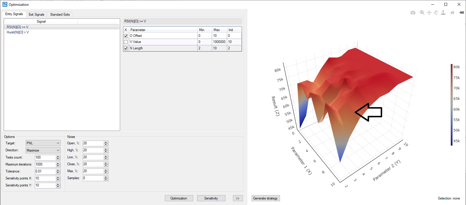
In this 3D chart, the parameter choices are $X=9$ and $Y=4$, as indicated by the black dot. Clearly, this area is near a sensitive region where strategy performance drops sharply. Following traditional recommendations, we should choose parameters $X=8$ and $Y=8$, where the graph is flatter.

In many cases, the parameter plateau hint is correct—because the parameters we choose are essentially functions of price changes; however, they are not price changes themselves. The most direct approach is that if strategy performance remains on a flat surface even when prices change slightly, it better demonstrates the robustness of the strategy.

However, such charts are difficult to plot. Therefore, BuildAlpha plots a 3D chart with parameters as coordinates in n-dimensional space and strategy performance as the value, but it is no longer based on a single historical dataset. Instead, it is based on a set of historical data: real historical data and data with added noise. In this context, the optimal parameters selected based on the parameter plateau will be more reliable.

This article references two articles from the BuildAlpha website, Noise Test Parameter Optimization and Noise Testing, and thanks Nelson for their assistance.