
Quantide Weekly: UO Indicator & FFT Factor Insights
This Week’s Highlights
- Nvidia and Sherwin-Williams added to the Dow Jones Industrial Average
- Manufacturing PMI returns to expansion territory after 5 months
- Q3 earnings season concludes; 80% of listed companies report profits
Next Week’s Watchlist
- Tuesday: US Election Day (Eastern Time)
- Tuesday: Caixin releases October Services PMI
- Nov 4–8: Standing Committee of the National People’s Congress (NPC); incremental policy tools may be unveiled
- Saturday: National Bureau of Statistics releases October PPI/CPI data
This Week’s Selections
- A Family of Champions: The Man Who Turned $1 into $10 in a Year Invented the UO Indicator
- The World is a Wave Function: DC Component Differential Factor Achieves 15% Annualized Return
The Dow Jones Industrial Average (DJIA) announced the inclusion of Nvidia and global coatings supplier Sherwin-Williams. Nvidia will replace Intel, and Sherwin-Williams will replace Dow Inc.
The National Bureau of Statistics reported that the manufacturing PMI for October was 50.1%, a 0.3-point month-over-month increase. This marks the manufacturing PMI’s return to expansion territory after running below the critical 50% threshold for five consecutive months.
Statistical data shows that nearly 80% of listed companies achieved profitability in the first three quarters, with nearly 50% posting positive net profit growth. The consumer goods sector shows clear recovery trends, while high-tech manufacturing demonstrates resilience. Industries such as agriculture, forestry, animal husbandry, fisheries, non-bank financials, electronics, and social services lead in net profit growth, with year-on-year increases of 507%, 42%, 37%, and 30%, respectively.
The Standing Committee of the National People’s Congress (NPC) will convene in Beijing from November 4 to 8. The one-time additional debt quota and “more than just this” incremental policy tools mentioned earlier by the Ministry of Finance may be unveiled during this session.
The “10x-in-a-Year” Man Invented the UO Indicator
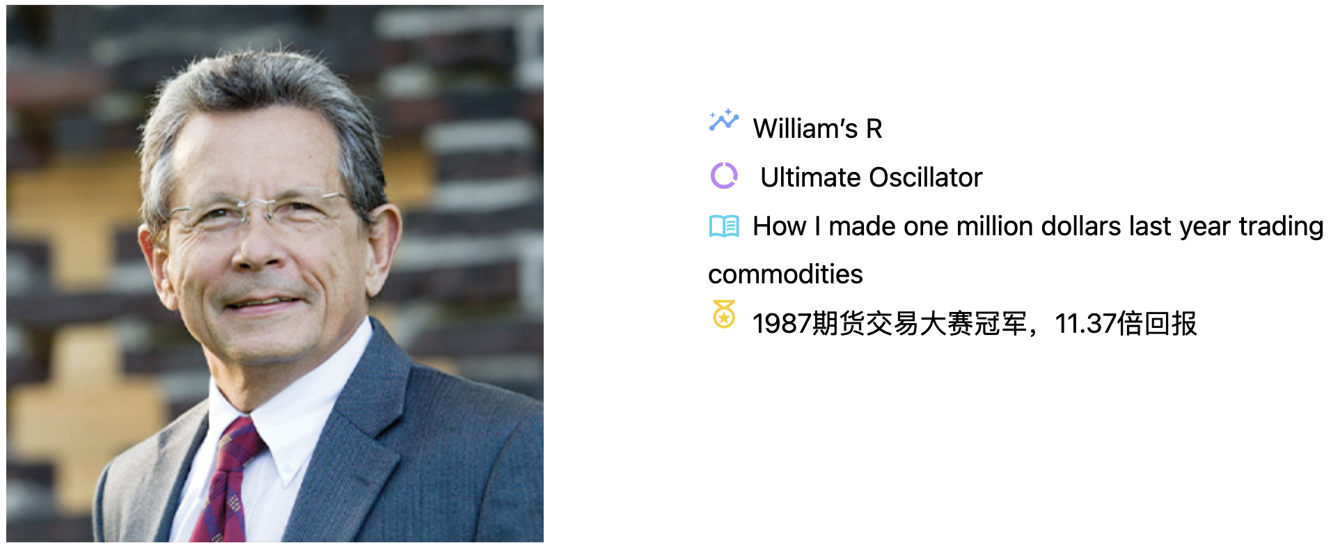
The Ultimate Oscillator (UO) is a technical analysis factor published by Larry Williams in 1976.
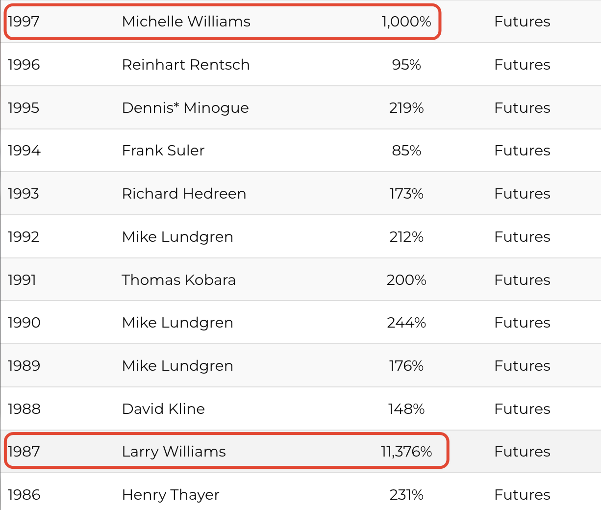
Larry is a serious practitioner, not just a talker. He invented two indicators: Williams %R (WR) and the Ultimate Oscillator. He is also the author of How I Made a Million Last Year Trading Futures. Furthermore, he was the champion of the 1987 World Futures Trading Championship, achieving an 11.37x return.
More impressively, the Williams family is a “triple crown” of trading excellence.
 Michelle Williams
This is his daughter, Michelle Williams. She is a renowned actress, starring in films such as Brokeback Mountain, and has received four Academy Award nominations for Best Supporting Actress. Remarkably, she also won the 1997 World Futures Trading Championship, securing a 10x return. In the history of this championship, only three individuals have achieved such returns; the Williams family accounts for two of them.
This demonstrates that the trading techniques of the elder Williams remain highly effective even after a decade.
Larry Williams’ son is a psychologist and the author of The Psychological Edge in Trading. With two world champions in his household, he certainly has no shortage of material for his writing.
Here is the calculation formula for the indicator.
$$ \text{True Low} = \min(\text{Low}, \text{Previous Close}) \ \text{True High} = \max(\text{High}, \text{Previous Close}) \ \text{BP} = \text{Close} - \text{True Low} \ \text{True Range} = \text{True High} - \text{True Low} \ \text{Average BP}n = \frac{\sum{i=1}^{n} BP_i}{\sum_{i=1}^nTR_i} \ ULTOSC_t=\frac{4Avg_t(7) + 2Avg_t(14) + Avg_t(28)}{4+2+1} \times 100 $$
The indicator aims to provide more reliable overbought and oversold signals by reducing false signals through the combination of buying pressure across different time horizons. The Ultimate Oscillator considers three different time periods, typically 7, 14, and 28 days, to capture short-term, medium-term, and long-term market momentum.
The calculation steps are somewhat complex, involving concepts such as true low, true high, true range, and bull power.
The following diagram clarifies the explanation.
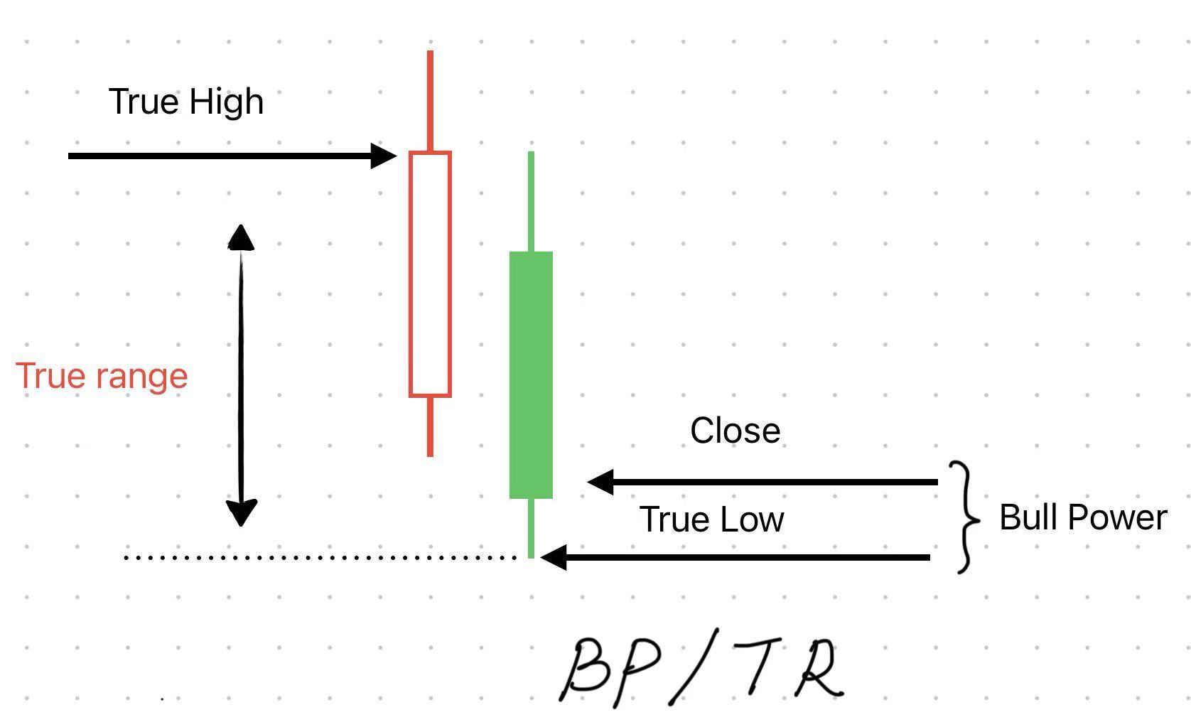
The so-called “true range” incorporates the previous close alongside the day’s high and low to calculate the maximum amplitude. It then calculates the price increase from the true low to the current price, serving as a measure of bullish power (Bull Power).
Finally, by dividing the bullish power by the true range and averaging over a specific window, we obtain the normalized average bullish power.
Ultimately, the indicator combines averages from long, medium, and short periods to generate the final value.
From a construction perspective, the most significant difference between UO and RSI is the inclusion of high and low price series data.
Traders know that the highest and lowest prices at critical moments are determined by the博弈 (game/struggle) between bulls and bears, embedding important information. Those who monitor the order book in real-time feel this even more deeply.
For instance, the highest price represents the amount of chips a major player buys in one go to push the price up. If the chips above cannot be absorbed, the highest price is set there. The unabsorbed chips represent the cost basis or other psychological price levels of larger capital, constituting future resistance levels.
Therefore, the Ultimate Oscillator contains more information than RSI. We hope this interpretation inspires future factor exploration.
The following figure demonstrates what the UO indicator looks like in practice. Visually, it resembles RSI, oscillating within a certain range.
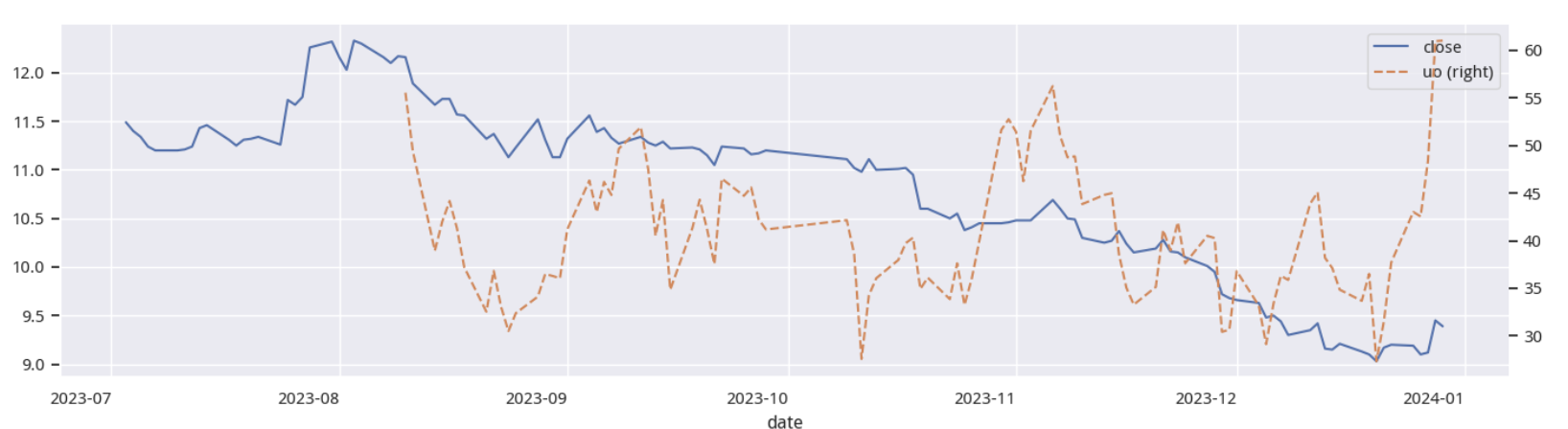
How does this factor perform in backtesting? From 2018 to 2023, over six years, its annualized alpha reached 13.7%, showing excellent performance.
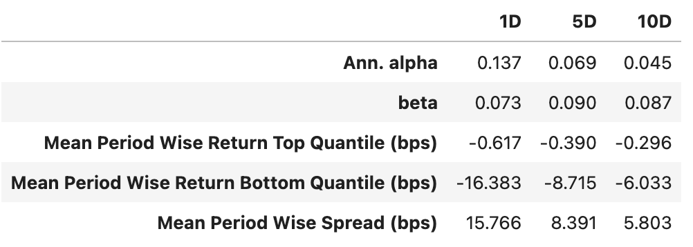
However, the factor’s returns are primarily driven by short positions. As seen in the layered return chart, returns are mainly contributed by shorting in Layer 1. Under a pure long-only strategy, the alpha is modest at only 1.6%, with returns largely driven by beta, resulting in higher portfolio volatility.
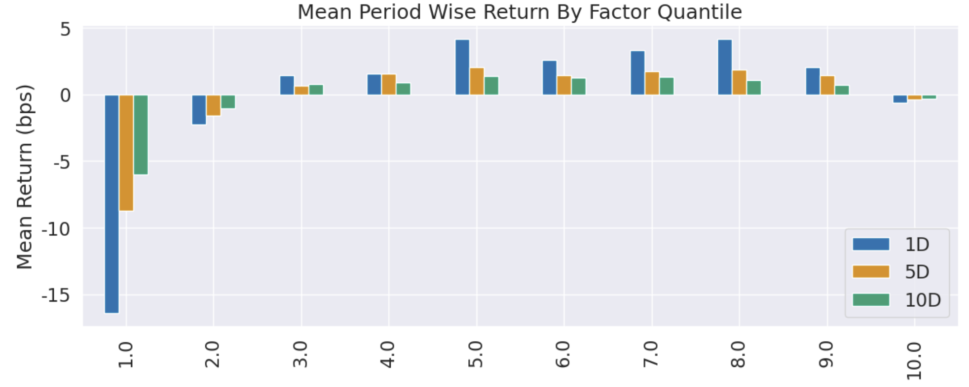
Thus, this indicator performs better in futures markets.
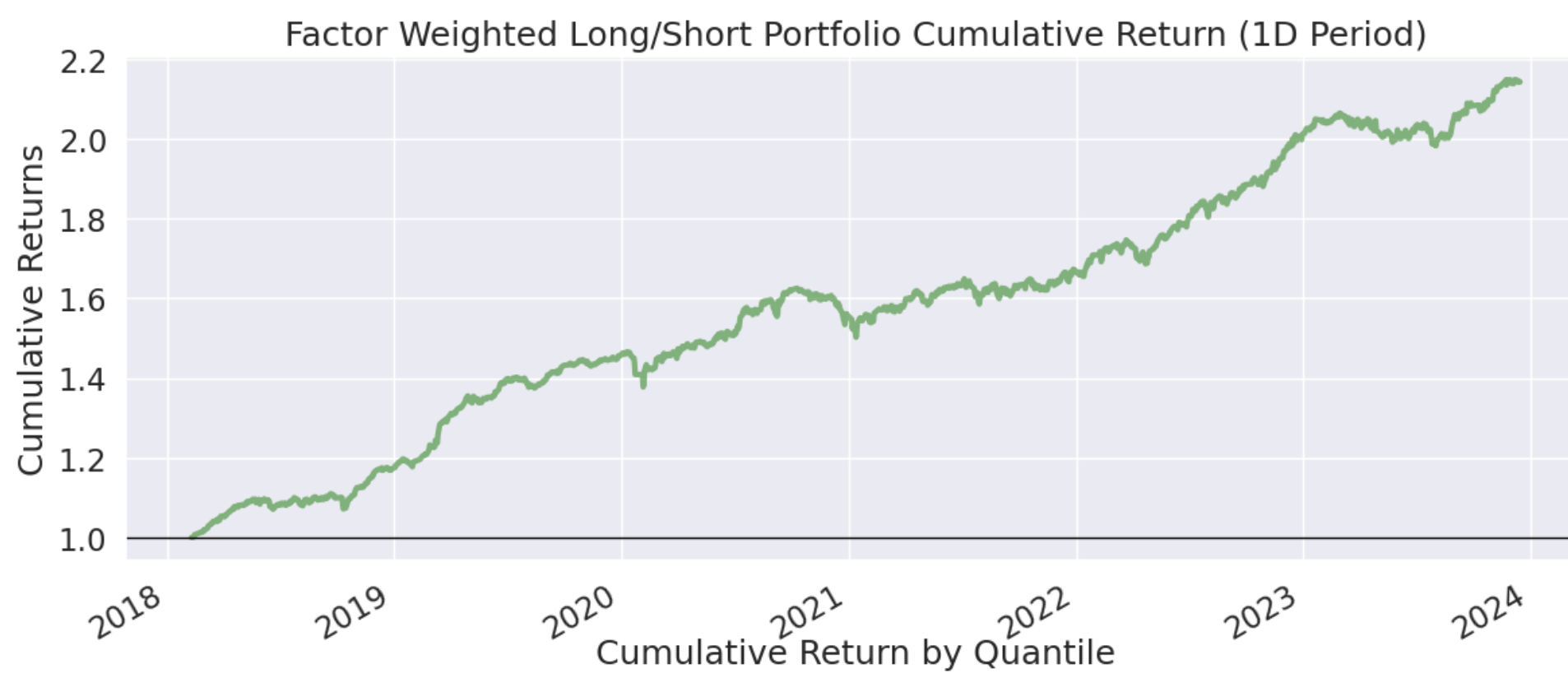
Under a long-short portfolio, the six-year return reached 2.2x.
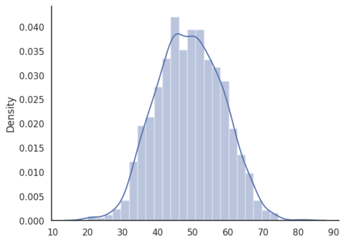
Finally, let’s look at the factor density distribution. It appears to follow a normal distribution, showcasing symmetric beauty.
From the layered mean return chart, we can make minor optimizations in trading, such as eliminating factors in Layer 8 and above. After this adjustment, the annualized alpha from 2018 to 2022 reached 24%, with a cumulative 5-year return of 2.75x.
We retained 2023 data as out-of-sample data for testing. In the 2023 backtest, the annualized alpha reached 13%, indicating no overfitting. The cumulative return curve for 2023 is as follows:
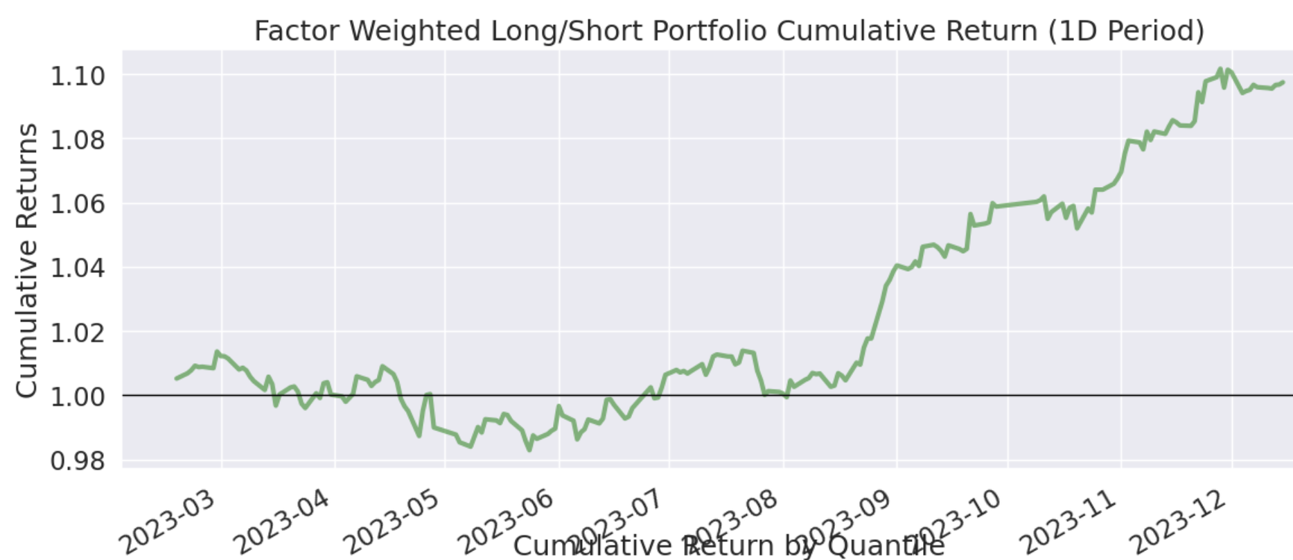
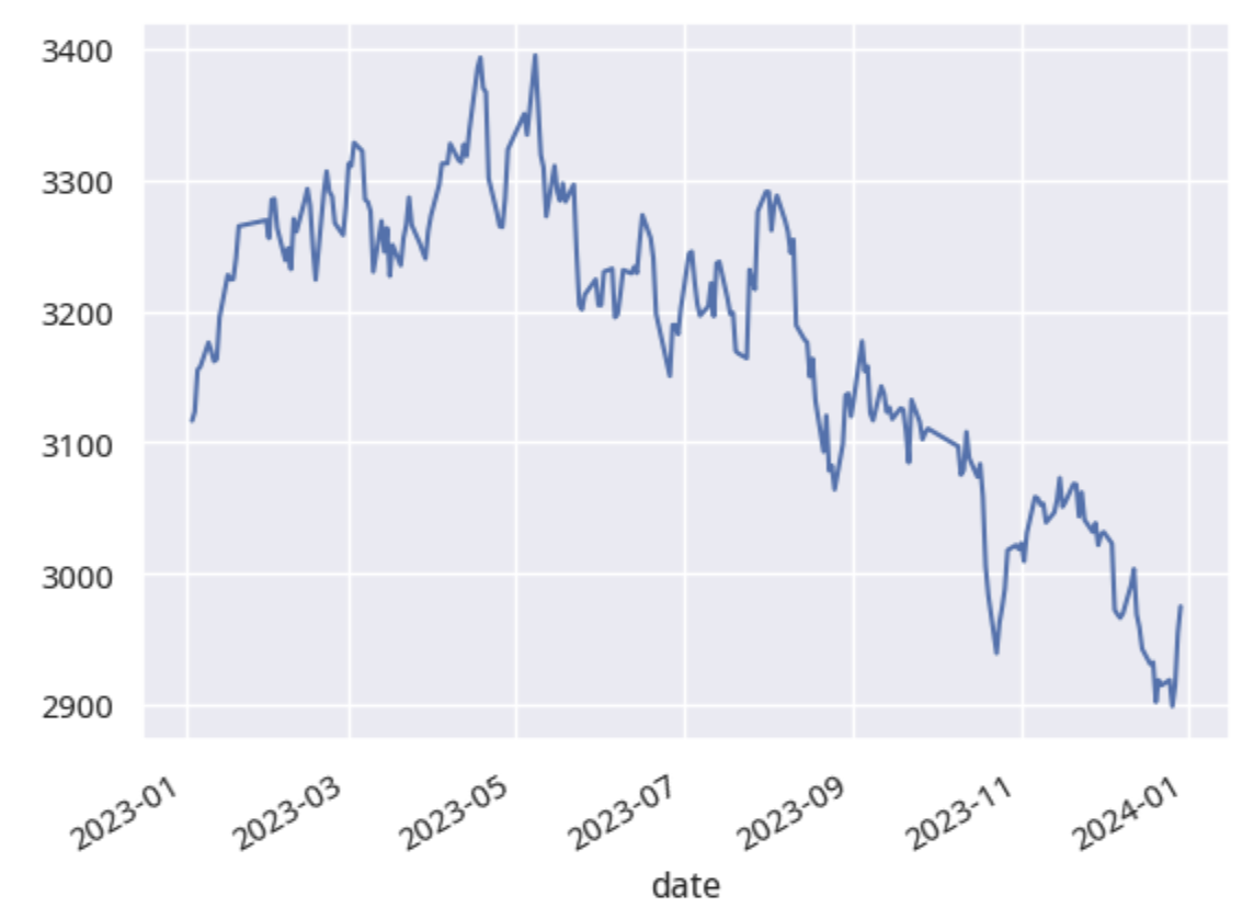
During the same period, the Shanghai Composite Index was predominantly in decline. The rally starting in late August coincidentally aligned with the timing of DMA strategy gains.
The World is a Wave Function
Intuitively, constructing factors using spectral analysis methods is natural, as economies and trading are cyclical. However, applying spectral analysis in quantitative trading presents challenges.
Take human voice spectral analysis: its frequency and energy ranges are fixed, meaning they are stationary sequences. Security prices, however, are not. As we have stated multiple times, stock prices are random sequences with an upward trend, driven by national economic development; thus, they are non-stationary.
Yet, we can always find methods to analyze such problems.
Spectral Transformation
Let us briefly introduce spectral transformation.
fft_result = np.fft.fft(close)
freqs = np.fft.fftfreq(len(close))
# Inverse Fourier Transform
filtered = fft_result.copy()
filtered[20:] = 0
inverse_fft = np.fft.ifft(filtered)
inversed = pd.Series(inverse_fft.real, index=close.index)# Plot original signal and decomposed signal
plt.figure(figsize=(14, 7))
plt.plot(close, label='Original Close')
plt.plot(inversed, label='Reconstructed from Sine Waves')
plt.legend()The first line transforms the time series into a spectrum, known as time-frequency transformation. The result is a complex array where the real part is the spectrum and the imaginary part represents the phase shift.
The array is sorted by frequency from low to high, meaning the beginning of the array contains low-frequency signals, and the end contains high-frequency signals. The element values represent the energy of the signal. Generally, high-frequency signals are treated as noise. In this array, the zeroth element has special significance: its frequency is zero Hertz, representing a DC component.
The first line generates the frequency codes, which depend only on the length of the time series. For a sequence of 30 time units, the highest frequency is considered 30 cycles. Whether a signal actually exists at that frequency depends on the value in the corresponding position of the previous array; if non-zero, the wave at that frequency exists.
Lines 6–8 perform simple processing on the transformed frequency signal by setting elements after index 20 to zero, achieving filtering.
We then use the inverse fast Fourier transform (IFFT) to convert the processed signal back and reconstruct the time series.
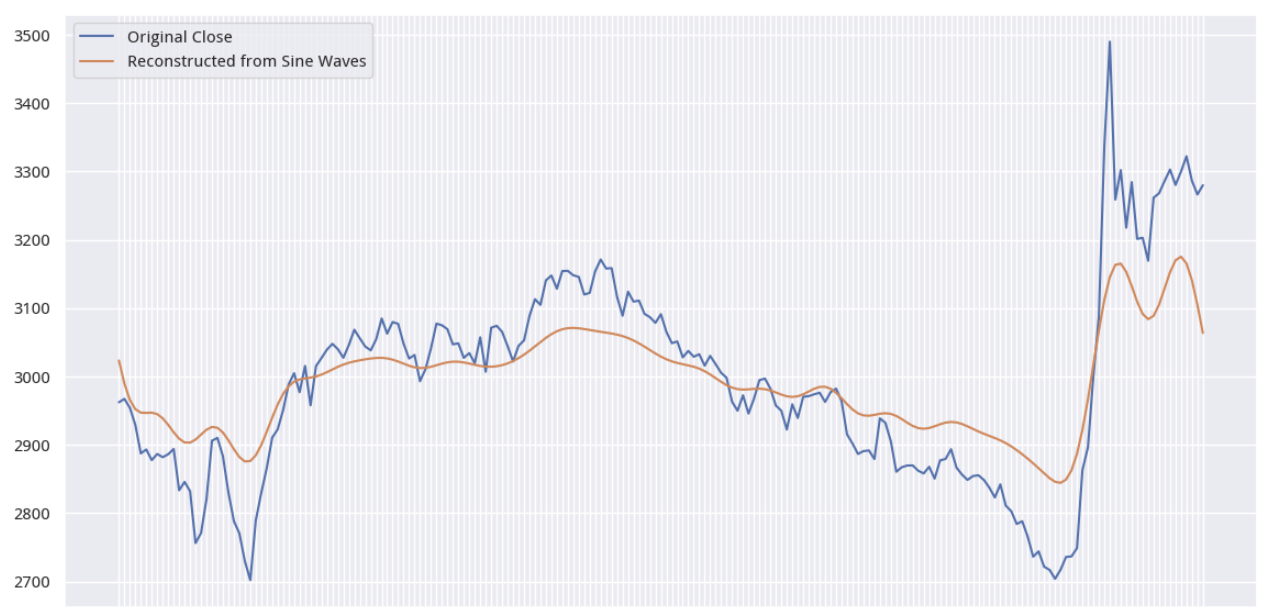
We observe that the image is smoother. Thus, this is also a method of moving average smoothing. This concludes our introduction to FFT.
Interpreting the DC Component
Now, let’s consider a question: what does the DC component obtained from time-frequency transformation of a price sequence signify?
Here is a hypothesis: if we view one vibration as one trade—buying causes the stock price to rise, and selling causes it to fall back to the starting point—this constitutes a vibration, right?
High-frequency vibrations correspond to high-frequency trading, while low-frequency vibrations correspond to low-frequency trading. Funds that do not trade within the window period are long-term capital, represented by the DC component in the signal. The greater the energy of the DC component, the smaller the energy of high-frequency vibrations, and the more stable the stock price.
Further, if the energy of the DC component at time $t_0$ is $e_0$, and at time $t_1$ it becomes $e_1$, what does the difference between the two signify?
It signifies that new long-term capital (exceeding the window period) has entered. Consequently, the stock price should be bullish.
DC Component Differential Factor
The principle of this factor is to treat stock prices as a fluctuation, perform spectral analysis using a 30-day sliding window, extract the DC component (the component with frequency 0), and use the differential of this component as the factor.
def calc_wave_energy(df, win):
close = df.close / df.close[0]
dc = close.rolling(win).apply(lambda x: np.fft.fft(x)[0])
return-1 * dc.diff()
np.random.seed(78)
_ = alphatest(2000, start, end, calc_factor=calc_wave_energy, args=(30,), top=9)Here is the annualized alpha. Surprisingly, we achieved a 17% annualized return:
| 1D | 5D | 10D | |
|---|---|---|---|
| Ann. alpha | 0.170 | 0.144 | 0.114 |
| beta | 0.022 | 0.030 | 0.040 |
| Mean Period Wise Return Top Quantile (bps) | 2.742 | 2.512 | 2.042 |
| Mean Period Wise Return Bottom Quantile (bps) | -9.614 | -8.516 | -7.270 |
| Mean Period Wise Spread (bps) | 12.355 | 11.178 | 9.473 |
Let’s look at the layered mean return chart. We have never seen such a perfect graph. It looks almost synthetic.
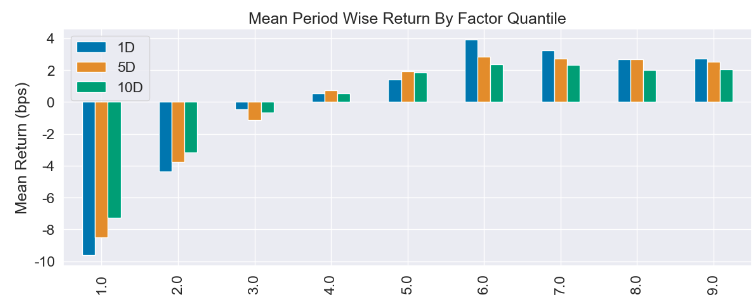
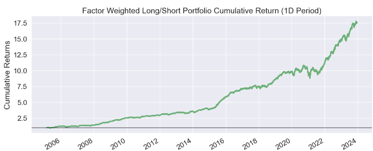
Cumulative returns over nearly 20 years reached 17.5x.
In our Factor Analysis and Machine Learning course, we disclose more high-efficiency factors and explain in depth the principles of factor analysis and machine learning for building quantitative trading strategies. Come join us in learning!