
Static vs Dynamic Adjustments: Why Your Factors Fail
Adjusting stock price data is a fundamental concept. You likely know there are two basic adjustment methods: forward adjustment (pre-split/dividend adjustment) and backward adjustment (post-split/dividend adjustment), as well as dynamic forward adjustment. However, most quantitative courses teach you how to calculate these adjustments but fail to explain how they impact your strategies.
In short, dynamic forward adjustment is the method closest to live trading. It perfectly replicates the most authentic prices seen at every point in time during the backtest, just as you would see them in live trading after deploying the strategy.
But dynamic forward adjustment does not mean adjusting only the transaction prices. Have you considered what happens to your strategy if you fail to adjust the factors accordingly?
What Is Dynamic Forward Adjustment?
Dynamic forward adjustment involves performing forward adjustment independently at every backtest time point $T_1, T_2, ..., T_n$. It corresponds to the following pseudocode:
for i in range(len(prices)):
qfq(prices[:i])Many backtesting frameworks do not support dynamic forward adjustment. For instance, in backtrader, we typically add market data as a data source during strategy initialization and perform adjustment at that stage. We then call the backtrader indicator system to calculate strategy indicators, or potentially introduce custom factors. Other frameworks operate similarly.
Finally, in the next method, the framework passes data to us, where the resulting factors and market data are calculated based on the adjusted data.
The problem is that frameworks like backtrader use static adjustment, meaning adjustment is based on a single fixed point in time for the entire backtest period. If using forward adjustment, the adjustment factor from the last day is applied backward; if using backward adjustment, the factor from the first day is applied forward. This means the data and indicators seen at time $t$ during the backtest differ from those in live trading (i.e., if you had studied this stock at some past time $t$, the indicators you calculated then would differ from those calculated during the backtest using static adjustment).
What if we perform forward adjustment ourselves within the next method? This would indeed be dynamic forward adjustment, perfectly replicating the live trading environment at that moment. However, implementing dynamic forward adjustment presents significant performance challenges.
In the pseudocode above, the adjustment process is called len(prices) times, with the input price sequence length increasing sequentially over time. Static forward adjustment, by contrast, is equivalent to calling qfq(prices) only once. Given modern CPU parallel computing capabilities, the latter is far faster than the former.
Moreover, after dynamically adjusting prices, we must also dynamically adjust the factors. Due to the nature of forward adjustment, historical data cannot be reused (therefore, storing forward-adjusted factor data in a database is meaningless); we must discard it and recalculate everything from scratch. Considering the massive volume of factor data and the complexity of calculations, this leads to severe performance issues.
However, before diving into the performance problems of dynamic forward adjustment, let’s first ask: is it truly necessary to calculate factors based on dynamic forward adjustment?
Why Must Factors Also Be Dynamically Forward Adjusted?
The slope factor is commonly used in various momentum strategies. Its calculation principle involves applying a sliding window to prices and calculating the slope of the price sequence within that window. We will use this as an example to demonstrate the necessity of dynamic factor adjustment.
If factor values remain consistent across different adjustment methods, we would not need dynamic forward adjustment. Conversely, inconsistency proves its necessity.
The following code calculates the slope values for each period under forward adjustment, backward adjustment, and dynamic forward adjustment.
import numpy as np
import pandas as pd
import matplotlib.pyplot as plt
random.seed(42)
pct_change = np.random.normal(0, scale=0.02, size=200)
price = np.cumprod(1 + pct_change).round(2)
# Generate a sequence that is not strictly monotonically increasing; its cumprod serves as a good sample for adjustment factors
f = np.array(random.sample([0, 0.01, 0.02], counts=[130, 50, 20], k = 200))
adjust = (1 + f).cumprod()
adjust[:10]
# Unified slope factor calculation function
def slope(ts, win):
x = np.arange(len(ts))
y = ts
coef = np.polyfit(x, y, 1)
return coef[0]
def slope_with_static_qfq(prices, adjust, win):
# Forward adjust the entire price sequence
qfq_prices = price * adjust / adjust[-1]
slopes = [slope(qfq_prices[i-win:i], win) for i in range(win, len(price))]
return np.array(slopes)
def slope_with_hfq(prices, adjust, win):
# Backward adjust the entire price sequence
hfq_prices = price * adjust / adjust[0]
slopes = np.array([slope(hfq_prices[i-win:i], win) for i in range(win, len(price))])
return np.array(slopes)
# Calculate slope under dynamic forward adjustment, which is what we truly see in live trading
def slope_with_dyn_qfq(prices, adjust, win):
slopes = []
for i in range(win, len(prices)):
ts = prices[i-win:i] * adjust[i-win:i] / adjust[i]
s = slope(ts, win)
slopes.append(s)
return np.array(slopes)
df = pd.DataFrame({
"static_qfq": slope_with_static_qfq(price, adjust, 5),
"static_hfq": slope_with_hfq(price, adjust, 5),
"dyn_qfq": slope_with_dyn_qfq(price, adjust, 5),
}, index=range(5, len(price)))
df.plot()
df.describe()The final output yields three curves:
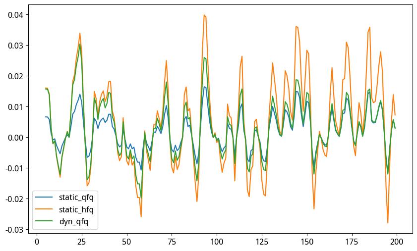
Do you see the problem?

Because there is only one "truth"! Yet we obtained three! This is the issue.
Compared to the unique true value (dynamic forward adjustment), backward adjustment amplifies the volatility of the slope, while forward adjustment shrinks it. If we extend the timeline further, the absurdity of forward and backward adjustment factors becomes even more apparent:
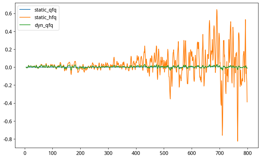
In this chart, as time progresses, the volatility of the backward-adjusted slope increases. Conversely, the further back we go, the smaller the volatility of the forward-adjusted slope becomes. What does this imply?
We separately took slope factors for 200, 400, and 800 periods, and calculated their volatility, resulting in the following table:
| static_qfq | static_hfq | dyn_qfq | |
|---|---|---|---|
| 200 | 0.86% | 2.09% | 1.12% |
| 400 | 0.39% | 2.33% | 0.69% |
| 800 | 0.38% | 13.55% | 1.01% |
Clearly, only the volatility of dynamic forward adjustment remains largely unaffected by the statistical period. The longer the statistical period, the higher the volatility of the backward-adjusted slope factor; the shorter the statistical period, the lower the volatility of the forward-adjusted factor.
This indicates that slope factors under both static adjustment modes are not time-stationary. For a non-time-stationary factor, it is practically impossible to utilize its statistical properties.
Only by basing calculations on dynamic forward adjustment can we state: "Over the past ten years, whenever the slope exceeded $x$, the stock price rose by so much; and when the slope was below $x$, the stock price fell by so much." If we use slope factors calculated via the other two methods, no approach can learn the relationship between these factors and returns.
However, if factors must be constructed based on dynamic forward adjustment data, the factor library becomes invalid (due to massive storage requirements); and real-time calculation during runtime, whether for backtesting or live trading, faces immense computational pressure.
Is there a better solution?
Performance Traps and an Elegant Solution
The answer is yes, but we need to split factor calculation into two steps. The result of the first step can be stored in the factor library; although it is not yet a dynamically forward-adjusted factor, it can be converted into one through a simple, fast calculation.
Let us first perform some mathematical derivation to prove the feasibility of this approach. We continue to use the slope factor as an example.
For forward-adjusted factors, the calculation formula is:
$$ Slope = Cov(X, P')/Var(X) \tag 1 $$
Here, $P'$ is the forward-adjusted price from time $T_0$ to $T_t$. $X$ is the sequence $range(0, t)$. Based on the forward adjustment formula:
$$ P' = P * adjust/adjust_{[-1]} \tag 2 $$
Substituting into equation 1), we obtain the dynamic forward-adjusted slope factor for period $t$:
$$ \begin{align} Slope_t &= Cov(X, P * adjust/adjust_{[-1]}) / Var(X) \tag 3 \ &= \frac{1}{adjust_{[-1]}}Cov(X, P * adjust) / Var(X) \tag 4 \ &= \frac{1}{adjust_{[-1]}}Cov(X, P * \frac{adjust}{adjust_0} * adjust_0) / Var(x) \tag 5 \ &= \frac{adjust_{0}}{adjust_{[-1]}}Cov(X, P * adjust/adjust_0) / Var(X) \tag 6 \ &= \frac{adjust_{0}}{adjust_{[-1]}}Slope_{hfq} \tag 7 \ \end{align} $$
Where $$ Cov(X, P * adjust/adjust_0) / Var(X) \tag 8 $$
is the backward adjustment formula.
Thus, we have established a bridge between backward-adjusted and dynamically forward-adjusted slope factors. Note that in equation 7), for any moment $t$, $adjust_0$ is a constant representing the adjustment factor at the start of the backtest; while $adjust_{[-1]}$ is the adjustment factor at time $t$.
Therefore, the dynamically forward-adjusted slope for each period equals the backward-adjusted slope factor multiplied by $adjust_0/adjust$. Here, $adjust$ is the adjustment vector containing all adjustment factors from the backtest start time to the current time $t$.
This yields a dynamically forward-adjusted factor calculation scheme with performance comparable to static adjustment. It adds only $n$ (where $n$ equals the backtest period) multiplication operations compared to static adjustment, a negligible time cost.
Now, let us verify whether the above derivation is correct. If the formula is valid, we can calculate dynamic forward adjustment as follows:
from numpy.testing import assert_array_almost_equal
# Calculate backward-adjusted factor
hfq_slope = slope_with_hfq(price, adjust, 5)
# Adjust to dynamic forward adjustment
actual = hfq_slope * adjust[0] / adjust[5:]
expect = slope_with_dyn_qfq(price, adjust, 5)
assert_array_almost_equal(actual, expect, decimal=5)Verification passed!
Can all factors be calculated first as backward-adjusted factors, then multiplied by $adjust[0]/adjust[t]$ to obtain dynamically forward-adjusted factors?
Common Factor Adjustment Formulas
Different factors require different adjustment methods.
1. Moving Average (MA)
$$ \begin{align} MA_{dyn}(t) &= Mean(P') \ &= Mean(P * adj/adj_{t}) \ &= Mean(P * adj/adj_0 * adj_0/adj_{t}) \ &= \frac{adj_0}{adj_{t}}Mean(P * adj/adj_0) \ &= \frac{adj_0}{adj_{t}}MA_{hfq}(t) \ \end{align} $$
Thus, to calculate a moving average factor based on dynamic forward adjustment, we only need to first calculate the sequence based on the benchmark adjustment, then compute the moving average (based on benchmark adjustment), and finally divide it by $\frac{adj_0}{adj_{t}}$.
2. Volatility (StdDev)
$$ \begin{align} Vol_{dyn}(t) &= \text{Std}(P') && \text{(1. Define dynamic volatility)} \ &= \text{Std}(P \cdot adj / adj_{t}) && \text{(2. Substitute price definition)} \ &= \frac{1}{adj_{t}} \text{Std}(P \cdot adj) && \text{(3. Extract constant factor)} \ &= \frac{1}{adj_{t}} \text{Std}\left(\frac{P \cdot adj}{adj_0} \cdot adj_0\right) && \text{(4. Introduce benchmark adjustment factor)} \ &= \frac{adj_0}{adj_{t}} \text{Std}\left(\frac{P \cdot adj}{adj_0}\right) && \text{(5. Extract constant factor again)} \ &= \frac{adj_0}{adj_{t}} \text{Std}(P_{hfq}) && \text{(6. Identify backward-adjusted price)} \ &= \frac{adj_0}{adj_{t}} Vol_{hfq}(t) && \text{(7. Identify backward-adjusted volatility)} \end{align} $$
The adjustment method is the same as for moving averages. If variance is used as the factor, the adjustment coefficient becomes $(adj_0/adj_{t})^2$.
3. Dimensionless Factors
Some dimensionless factors, such as RSI or Bollinger Bands, can be calculated based on static adjustment data and generally require no additional adjustment. Generally, if a factor is calculated based on price percentage changes, it has already eliminated the impact of adjustment methods, so dynamic adjustment is unnecessary.
Actually, for the slope factor, note that it is affected by absolute prices, leading to significant differences in slopes across different assets, making them incomparable. Therefore, to compare slope factors across the cross-section, we should dimensionless the prices (e.g., by dividing by $price_0$) to obtain relative prices, and then calculate the slope. In this case, the slope factor becomes dimensionless, allowing cross-asset comparison and eliminating the need for dynamic adjustment.
Synthesizing the above discussion, the key to using the two-step method to calculate dynamically forward-adjusted factors depends on the homogeneity of the factor calculation function. If the factor calculation function is linear (first-order homogeneous), the adjustment factor is the same as for MA/slope; if it is quadratic homogeneous, it is the same as for variance; dimensionless factors are zero-order homogeneous and require no adjustment.
If the factor calculation function is non-homogeneous, such as MACD, the two-step method cannot be used to calculate dynamically forward-adjusted factors. If the factor calculation function uses logarithms, the adjustment algorithm will be additive rather than multiplicative.
Therefore, specific adjustments must be determined after analyzing the mathematical properties of the factor calculation function.
Saving Your Factor Library
Based on the above discussion, we draw several important conclusions:
- Be cautious when using factor