This Week’s Highlights

• SSE Launches Total Return Index: To facilitate investor observation of overall market returns, the Shanghai Stock Exchange (SSE) and China Securities Index Co., Ltd. will officially release real-time data for the SSE Composite Total Return Index starting July 29. The index code and abbreviation have been adjusted to "000888" and "SSE Return," respectively.
  
  
• Private Funds Speak Out: DMA (Direct Market Access) holdings dropped by 200 billion RMB this week. Fuhang and Yanfu, prominent quantitative private funds, issued statements arguing that quantitative investing has long-term advantages and should not be viewed as the primary cause of market downturns. Since 2023, DMA strategies have performed well, becoming a key profit driver for private funds, yet they have also faced market criticism.
  
  
  
• Exchanges Tighten Oversight on Abnormal Trading: The Shenzhen Stock Exchange (SZSE) took self-regulatory measures against 54 instances of abnormal trading behavior this week. The SSE focused on monitoring convertible bonds with high volatility and issued written warnings against 49 cases of abnormal trading, such as price manipulation and false declarations. The Shanghai Futures Exchange (SHFE) also released the revised "Abnormal Trading Behavior Management Measures," effective October 25, 2024.
  
  
• Bitcoin Breaks $67,000: Bitcoin surged past $67,000 intraday.
  
  
• Short-Term Bond Funds Surge: The total scale of short-term bond funds has exceeded 800 billion RMB, a 50% increase in six months. Central Huijin continued to increase ETF holdings in Q2, with subscription amounts nearing 300 billion RMB. Equity ETF scales grew by over 420 billion RMB year-to-date, with broad-based ETFs driving the growth.
  
  
• Tesla Dips on Blue Screen News: Tesla shares fell nearly 5% intraday on Friday, closing down 4.02%, hit by the dual blows of Trump’s comments and the Microsoft/CrowdStrike blue screen incident.

---

Next Week’s Calendar

• Monday: The PBOC will announce July LPR quotes. Market expectations suggest a potential window for RRR cuts or rate cuts in Q3 or Q4 to further support steady economic growth.
  
  
• Monday: Short-selling margin ratios are raised to 100%, and for private securities investment funds participating in short selling, the margin ratio is raised from 100% to 120%. Notably, after the CSRC’s announcement, A-share short-selling scales have begun to decline continuously. Wind data shows that as of July 18, short-selling balances had decreased to approximately 29.5 billion RMB, hitting a four-year low.
  
  
• Starting July 24: Issuance of ultra-long-term special treasury bonds. This tranche consists of 30-year fixed-rate coupon bonds, with a competitive bidding face value total of 55 billion RMB.
  
  
• This Week: Three new IPOs will be issued: Liju Thermal Energy, Boshijie, and Longtu Optical Mask.
  
  
• This Friday: Refined oil price adjustment window. Calculations indicate a potential retail price reduction of 50 RMB/ton for domestic gasoline and diesel.
  

This Week’s Articles

We published five articles this week. A Portfolio Strategy Based on XGBoost... and another article detail the framework and common pitfalls of using machine learning to construct portfolio strategies.

---

Key Points and Conclusions:

1. A two-stage approach is used to construct multi-factor, multi-asset portfolio strategies. Stage one builds multiple single-asset multi-factor models using XGBoost; stage two performs portfolio optimization via classic mean-variance methods.
2. Machine learning models should be built based on classification rather than regression. Time-series price forecasting is largely meaningless (price series are non-stationary).
3. Classification models are trained using multi-factors as features and the digitized future one-period return magnitude as labels.
4. For XGBoost models, factor standardization is generally unnecessary. Factor standardization might even introduce side effects; however, it can also benefit regularization penalty terms.
5. The difference between loss functions and metric functions lies in gradient computation. The non-differentiability of MAPE makes it unsuitable as a loss function.
6. In finance, relative error is more meaningful than RMSE. Therefore, we introduce SMAPE—a function that can serve as a loss function.

We have compiled these two articles and placed them at the end of this piece.

In this week’s Quant Tools column, we published The Man Who Won the NASA Medal Brings These IPython Tips. IPython is a very lightweight interactive programming tool. Although all its features can be found in Notebooks, it is lighter yet highly versatile, possessing a certain elegance.

In Don’t Write Books Unless You Are Talking to Your Soul, we revealed some awkward moments during the publication of Python Efficient Programming Practice Guide. This book will be very helpful for quants building robust trading systems.

---

Just as we finished speaking, the Windows blue screen incident occurred on Friday. This happened precisely because CrowdStrike lacked a robust CI/CD pipeline, which is one of the key topics detailed in this book.

In Ask with Confidence: The Most Comprehensive Self-Study Roadmap for Quant, we introduced the quantitative self-study outline written by Algos.org.

We will also launch our own quantitative self-study roadmap by the end of August. In addition to better localization (in the English version, some tools, websites, and data sources do not support the domestic market), we will also clearly map out learning paths from beginner to expert, and from novice to different roles.

Until the outline is released, you can temporarily refer to this roadmap:

---

Building Multi-Factor Strategies with XGBoost

How can we apply machine learning methods to portfolio strategies? Recently, we reviewed some stored papers and decided to interpret the paper A Portfolio Strategy Based on XGBoost Regression and Monte Carlo Method.

Here is a basic framework diagram abstracted from the paper.

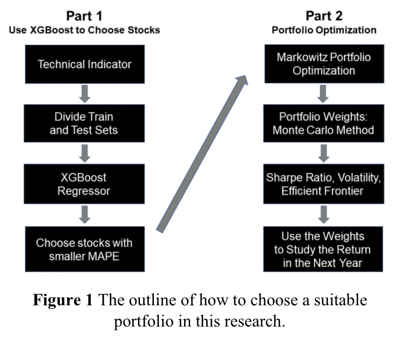
What problem does this framework solve? We know that in a portfolio strategy, the first key issue to consider is how to select a subset of stocks from a given universe to include in the strategy’s stock pool; the second is how to allocate positions among these stocks to achieve the highest risk-adjusted return for the portfolio.

---

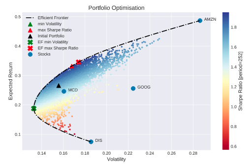
For the latter part, the most classic method is to use Modern Portfolio Theory (MPT) to find the efficient frontier. This can be solved using convex optimization or Monte Carlo methods. We previously had a series of articles on Portfolio Theory and Practice, which clearly covered everything from basic concepts to practical details, so we won’t elaborate here.

How to select stocks from the universe to enter the stock pool? This is relatively easy to solve in single-factor models: simply select stocks from the best-performing tier (layer) in factor ranking. Weights for each asset can be allocated based on factor loadings or using MPT methods.

But how to select stocks to enter the stock pool in a multi-factor model? This has always been a difficult problem. The Barra model we often mention is merely a risk control model and cannot select the optimal stock pool.

---

The paper’s approach is to view stock selection as a regression problem: train with multi-factors to identify those stocks that can be best predicted by the model to enter the stock pool.

The author’s results showed that the returns for the leading stock portfolios in 2021, 2020, and 2019 were 27.86%, 6.20%, and 23.26%, respectively. However, the author did not provide benchmark comparisons, nor did they deeply analyze whether any excess returns came from MPT or from XGBoost.

This is where we need to interpret this paper. We hope that through our interpretation, you can also learn how to analyze others’ papers and extract the correct parts.

The Flawed Regression

The paper uses an XGBoost regression model. This is questionable. In asset pricing models, we aim to predict the relative strength of stocks in the cross-section, not their time-series trends.

The author’s method here is to train a regression model to predict next-day (or subsequent period) trends well.

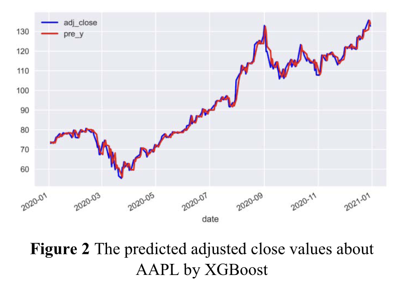
The right graph shows one of the results obtained by the paper’s author. It appears the model predicts next-day trends almost perfectly.

---

Obviously, since the XGBoost regression model itself lacks the ability to predict stock strength, even if a regression model identifies perfectly fitted stocks, it is meaningless. A declining stock can also be perfectly fitted. Therefore, the returns mentioned in the paper, even if they show excess returns, likely come from MPT theory.

However, the author still provides a clue on how to use XGBoost to find the best-performing individual stocks in a multi-factor model. We just need to transform it into a classification model and then filter out the best-performing stocks via the classification model.

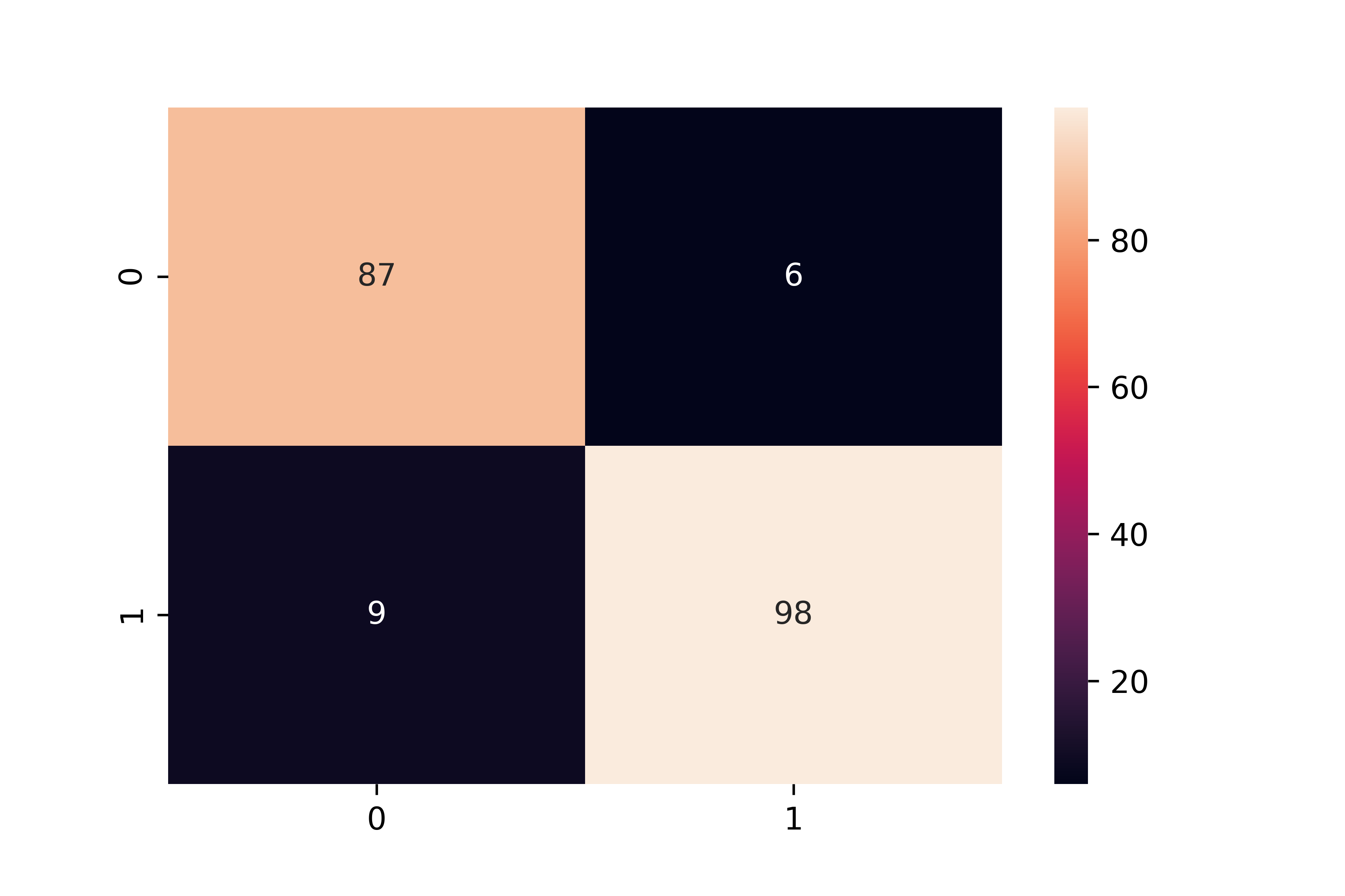
The X part in the training set does not need to change, but we need to redefine the labels, i.e., the y part. For a given factor $X_i$, the corresponding $y_i$ needs to reflect whether the stock is rising or falling. If possible, we can set the labels into 5 categories: -2 for a sharp drop, 2 for a sharp rise, and so on for the middle parts.

Then, construct a classifier for training. After training, stocks predicted to belong to the "sharp rise" label are included in the stock pool. Weights can be allocated equally or optimized via MPT theory.

End-to-End Training and New Network Architecture

The framework used by the paper’s author is two-stage: first, select stocks to enter the strategy pool, then optimize weights via MPT.

---

Even in the first stage, it is still two-stage. Each time it is trained, it only uses multi-factor data for a single asset. Therefore, if the universe contains 1,000 assets, 1,000 models must be trained (this is the method implied in the paper; alternatively, one model could be trained 1,000 times).

The reason for this is technical limitations. XGBoost only supports two-dimensional input. If we want to train multiple assets’ multi-factors simultaneously, we must use panel format data or flatten the multi-factors of multiple assets into one dimension. However, if the number of assets is too large, training after flattening becomes difficult.

Thus, due to technical constraints, we can either perform multi-asset single-factor simultaneous training or multi-factor single-asset training.

However, the paper’s author provides a method here: you can train models for each asset separately, perform predictions separately, and then evaluate via MAPE. When we change to a classification model, we can simply look at the classification results or combine classification metrics (in the time-series dimension) to select assets with both high accuracy and good classification results to include in the strategy stock pool.

Loss Functions vs. Metric Functions

Next, we need to analyze the use of the MAPE function in the paper. Using this as an opportunity, we will delve slightly deeper into machine learning principles to discuss two key points:

---

Loss Functions vs. Metric Functions

In machine learning, there are two types of important functions: one is the objective function (loss function), and the other is the metric function (metrics).

Loss functions are used for model training. During training, methods such as gradient descent are used to continuously reduce the value of the loss function until it can no longer decrease, at which point the model is trained.

---

The trained model is then tested on the test dataset, and the predicted results are compared with the true values. To quantify this comparison process, we introduce metric functions (metrics).

sklearn provides a large number of loss functions and metric functions. The following figure lists some of the loss functions and metric functions provided by Sklearn:

---

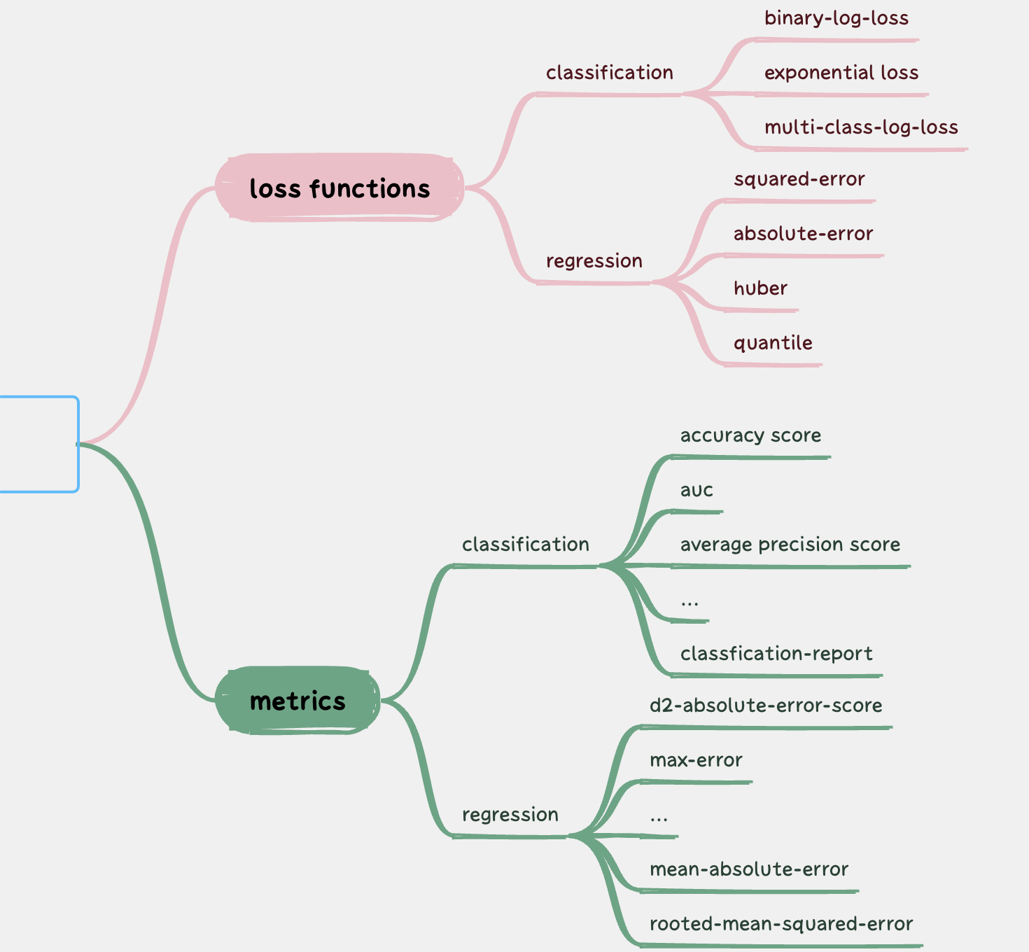
It can be seen that the number of metric functions is far greater than that of loss functions. Why is this?

---

In the paper, the author did not disclose the specific training process via XGBoost, only stating that the XGBoost database was used directly. This expression is somewhat strange; we can understand it as using the default values for XGBoost parameters.

---

However, the author重点 (key) mentioned using MAPE. From the process, it appears MAPE was used as a metric function for post-hoc evaluation.

In XGBoost, if no specific objective function is specified, the default is to use the RMSE (rooted mean square error) function with regularization penalties. RMSE can also serve as a metric function. In the paper, the author did not use RMSE as a metric function but chose MAPE (mean absolute percentage error). Why? If MAPE is better than RMSE in this scenario, why not use MAPE during training?

It seems that both objective functions and metric functions aim to make predicted values closer to true values. Given this shared characteristic, why distinguish between these two types of functions?

To answer these questions, we must understand XGBoost’s training principle: specifically, how it computes gradients.

XGBoost: Second-Order Taylor Expansion

XGBoost is a Boosting algorithm. It constructs a strong learner by stacking multiple weak learners. In each iteration, the new tree corrects the residuals of the existing model, i.e., the difference between predicted and true values. The magnitude of this difference is calculated by the objective function.

---

In XGBoost, the stacking of multiple weak learners adopts an additive model,

---

meaning the final prediction is the weighted sum of outputs from all weak learners. This model allows us to use Taylor expansion to approximate the loss function, thereby achieving efficient optimization.

XGBoost optimizes the objective function via second-order Taylor expansion and computing the second derivative. By using the second derivative, XGBoost can achieve faster convergence because it considers not only the direction of the gradient but also the shape of the loss function.

$$ f(x) \approx f(a) + f'(a)(x-a) + \frac{f''(a)}{2!}(x-a)^2 $$

It is precisely due to XGBoost’s internal optimization principle that the objective function we choose must be second-order differentiable.

RMSE is second-order differentiable, but MAPE is not: by definition, MAPE can take zero values. Near these zero points, even the first derivative does not exist, let alone the second derivative. The formula for MAPE is as follows:

$$

\text{MAPE} = 100\frac{1}{n}\sum_{i=1}^{n}\left|\frac{\text{Actual Value} - \text{Predicted Value}}{\text{Actual Value}} \right| $$

When the predicted value equals the actual value, the MAPE value becomes zero.

How to Choose the Objective Function?

Choosing MAPE as a metric function is not only convenient for comparing different models but also holds special importance in finance:

---

We care more about the relative error between predicted and true values than the absolute error. In trading, percentages are king. For this reason, if MAPE could be used as the objective function during training, the resulting prediction accuracy would be closer to practical applications than that achieved by training with RMSE.

This is an entry point for improving algorithms in specific domains. Someone has already invented a loss function called SMAPE, with the formula:

$$

\text{SMAPE} = \frac{100}{n} \sum_{t=1}^n \frac{\left|F_t-A_t\right|}{(|A_t|+|F_t|)/2} $$

So far, sklearn has not provided this function, but we can implement it ourselves and integrate it into the sklearn system via sklearn’s make_scorer method:

---

123456789101112from sklearn.metrics import make_scorer

def smape(y_true, y_pred):
    return np.mean(2.0 * np.abs(y_pred - y_true) / 
           (np.abs(y_true) + np.abs(y_pred)))

smape_scorer = make_scorer(smape, greater_is_better=False)

# 使用举例：在GridSearchCV中使用
grid_search = GridSearchCV(estimator=model, 
                           param_grid=params, 
                           scoring=smape_scorer)

Question: Since MAPE cannot be used in training, why did the author use MAPE in testing?

The answer is actually simple: it is for easier comparison across multiple models. In the author’s algorithm, each stock must have its own model. Since the absolute prices of different stocks vary, their RMSE values differ. MAPE, however, acts as a normalized indicator, allowing comparison across different models to ultimately select the model with the smallest error and include its corresponding stock in the strategy pool.

But as we mentioned earlier, the author’s model is meaningless; using a classification model would be better. If we switch to a classification model, the loss function is no longer RMSE, and the metric function cannot be MAPE.

---

Standardization

The paper also notes that the author standardized the factor data prior to training.

In reality, this step is largely superfluous. XGBoost is a decision tree-based model that splits and partitions data based on feature value comparisons. Since split points do not depend on the scale or units of the data, standardization is unnecessary and may even introduce precision loss, resulting in a net negative outcome.

That said, this is not a universal rule. XGBoost employs regularization to control tree complexity, including L2 regularization on leaf node weights. If you apply a **regularization penalty** to the loss function during XGBoost training without standardizing the features, the regularization effect may degrade.

Furthermore, the method described in the paper trains a separate model for each stock. What if we train a single model using data from 1,000 stocks, iterating 1,000 times? In this scenario, pre-standardization becomes mandatory.

Otherwise, convergence becomes difficult (though standardization does not guarantee convergence; success depends on whether many stocks share the same mapping from features to labels). This is not a requirement of XGBoost itself, but an additional constraint imposed by our specific usage pattern.

Conclusion

For most quantitative researchers, it is impractical to build a machine learning framework from scratch like Tianqi Chen. Therefore, to achieve superior results using the same models, we must focus on data labeling, objective functions, evaluation metrics, and parameter tuning. This approach typically requires deep domain expertise alongside a solid understanding of specific model mechanics.

Copyright: Quantitative Wind / QuanTide Official Account