
Automated Triangle Pattern Detection for Quant Trading
The final module of the Kuang Ti. Factor Analysis and Machine Learning Strategies course covers the application of deep learning frameworks in quantitative trading. Since many technical traders rely on chart patterns—such as Elliott Wave theory, head-and-shoulders formations, and triangle consolidations—it makes sense to leverage Convolutional Neural Networks (CNNs). Given that CNNs have surpassed human capabilities in image pattern recognition, this article uses triangle consolidation detection as a case study.
To implement triangle detection via a CNN, the first step is data annotation. We have already developed an annotation tool in the course. However, I aim to detect triangle patterns algorithmically. This article introduces that algorithm.

If you wish to access the source code for this article, you can join our private community. After three days of membership, you will gain access to our research platform, which hosts executable and verifiable notebook versions, allowing you to fully reproduce the results presented here.
note

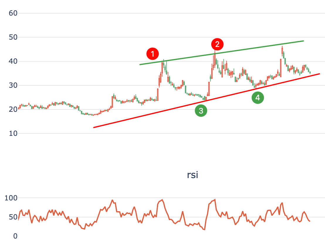 Triangle Detection Schematic
First, we must identify the peaks and valleys in the candlestick chart. In the diagram, points 1 and 2 are peaks, while points 3 and 4 are valleys. We then draw a line through points 1 and 2 to establish the resistance line, and another line through points 3 and 4 to establish the support line.
In Python, the line between two points can be calculated using np.polyfit. This function returns the slope of the line. By analyzing the relationship between the slopes of these two lines, we can further define the triangle's morphology.
Let $S_r$ denote the slope of the resistance line and $S_s$ denote the slope of the support line. The triangle's morphology can be defined by the following table:
| Resistance Direction | Support Direction | Angle Comparison | Flag | Description |
|---|---|---|---|---|
| $S_r > 0$ | $S_s > 0$ | $ | S_r | > |
| $S_r > 0$ | $S_s > 0$ | $ | S_r | < |
| $S_r > 0$ | $S_s < 0$ | $ | S_r | > |
| $S_r > 0$ | $S_s < 0$ | $ | S_r | < |
| $S_r < 0$ | $S_s > 0$ | $ | S_r | > |
| $S_r < 0$ | $S_s > 0$ | $ | S_r | < |
| $S_r < 0$ | $S_s < 0$ | $ | S_r | > |
| $S_r < 0$ | $S_s < 0$ | $ | S_r | < |
Some of these patterns are illustrated below:
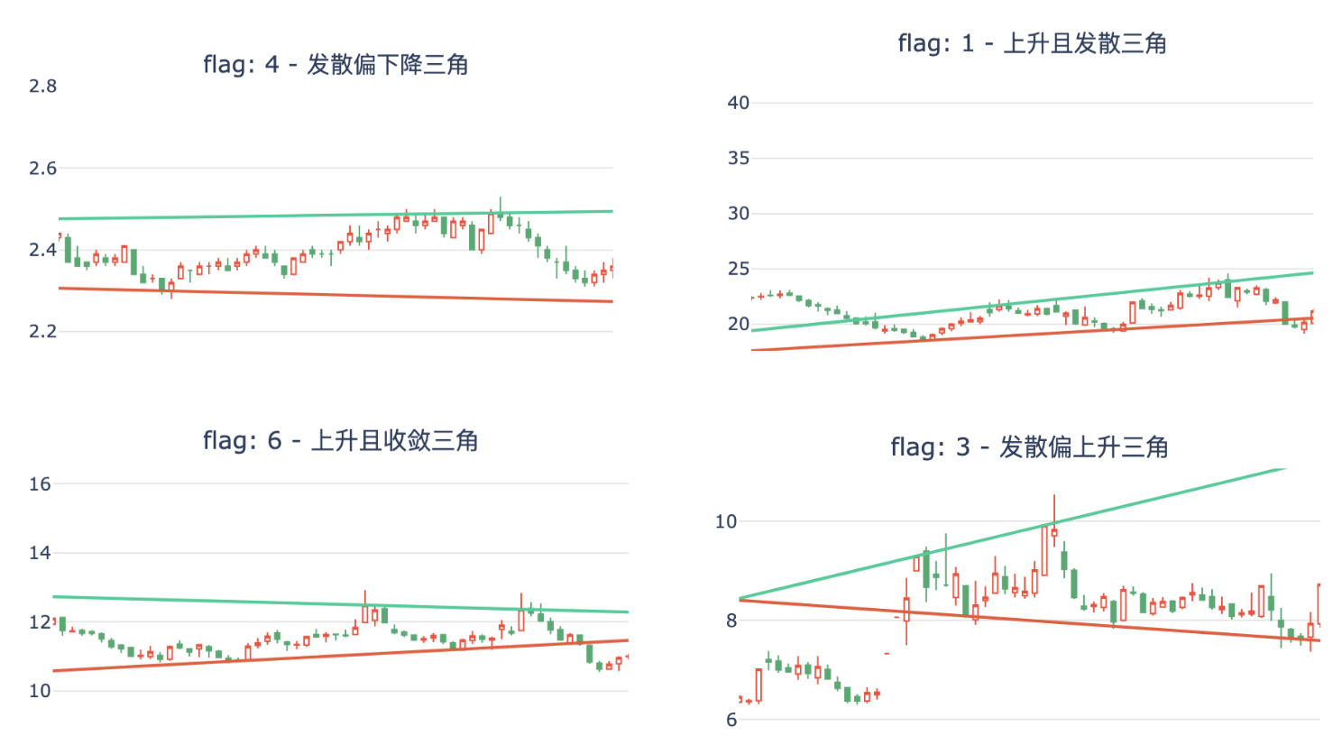
The implementation code for the identification algorithm is as follows:
from zigzag import peak_valley_pivots
def triangle_flag(df, lock_date=None):
if lock_date is not None:
peroid_bars = df.loc[:lock_date]
else:
peroid_bars = df
thresh = peroid_bars.close[-120:].pct_change().std() * 3
pvs = peak_valley_pivots(peroid_bars.close.astype(np.float64), thresh, -1 * thresh)
if len(pvs) == 0:
return 0, None, None
pvs[0] = pvs[-1] = 0
pos_peaks = np.argwhere(pvs == 1).flatten()[-2:]
pos_valleys = np.argwhere(pvs == -1).flatten()[-2:]
if len(pos_peaks) < 2 or len(pos_valleys) < 2:
return 0, None, None
minx = min(pos_peaks[0], pos_valleys[0])
y = df.close[pos_peaks].values
p = np.polyfit(x=pos_peaks, y=y, deg=1)
upper_trendline = np.poly1d(p)(np.arange(0, len(df)))
y = df.close[pos_valleys].values
v = np.polyfit(x=pos_valleys, y=y, deg=1)
lower_trendline = np.poly1d(v)(np.arange(0, len(df)))
sr, ss = p[0], v[0]
flags = {
(True, True, True): 1,
(True, True, False): 2,
(True, False, True): 3,
(True, False, False): 4,
(False, True, True): 5,
(False, True, False): 6,
(False, False, True): 7,
(False, False, False): 8,
}
flag = flags[(sr > 0, ss > 0, abs(sr) > abs(ss))]
return flag, upper_trendline, lower_trendlinedef show_trendline(asset, df, resist, support, flag, width=600, height=400):
desc = {
1: "Rising Divergent Triangle",
2: "Rising Convergent Triangle",
3: "Divergent Upward-Biased Triangle",
4: "Divergent Downward-Biased Triangle",
5: "Falling Convergent Triangle",
6: "Rising Convergent Triangle",
7: "Falling Convergent Triangle",
8: "Falling Divergent Triangle",
}
if isinstance(df, pd.DataFrame):
df = df.reset_index().to_records(index=False)
title = f"flag: {flag} - {desc[flag]}"
cs = Candlestick(df, title=title, show_volume=False, show_rsi=False, width=width, height=height)
cs.add_line("support", np.arange(len(df)), support)
cs.add_line("resist", np.arange(len(df)), resist)
cs.plot()
np.random.seed(78)
start = datetime.date(2023, 1, 1)
end = datetime.date(2023, 12, 29)
barss = load_bars(start, end, 4)
for key, df in barss.groupby("asset"):
df = df.reset_index().set_index("date")
flag, resist, support = triangle_flag(df)
if flag != 0:
show_trendline(key, df, resist, support, flag)Finally, let us examine a specific stock to explore the potential applications of this algorithm:
start = datetime.date(2023, 1, 1)
end = datetime.date(2023, 12, 29)
barss = load_bars(start, end, ("300814.XSHE", ))
for key, df in barss.groupby("asset"):
df = df.reset_index().set_index("date")
flag, resist, support = triangle_flag(df, datetime.date(2023, 9, 11))
if flag != 0:
show_trendline(key, df, resist, support, flag, width=800, height=600)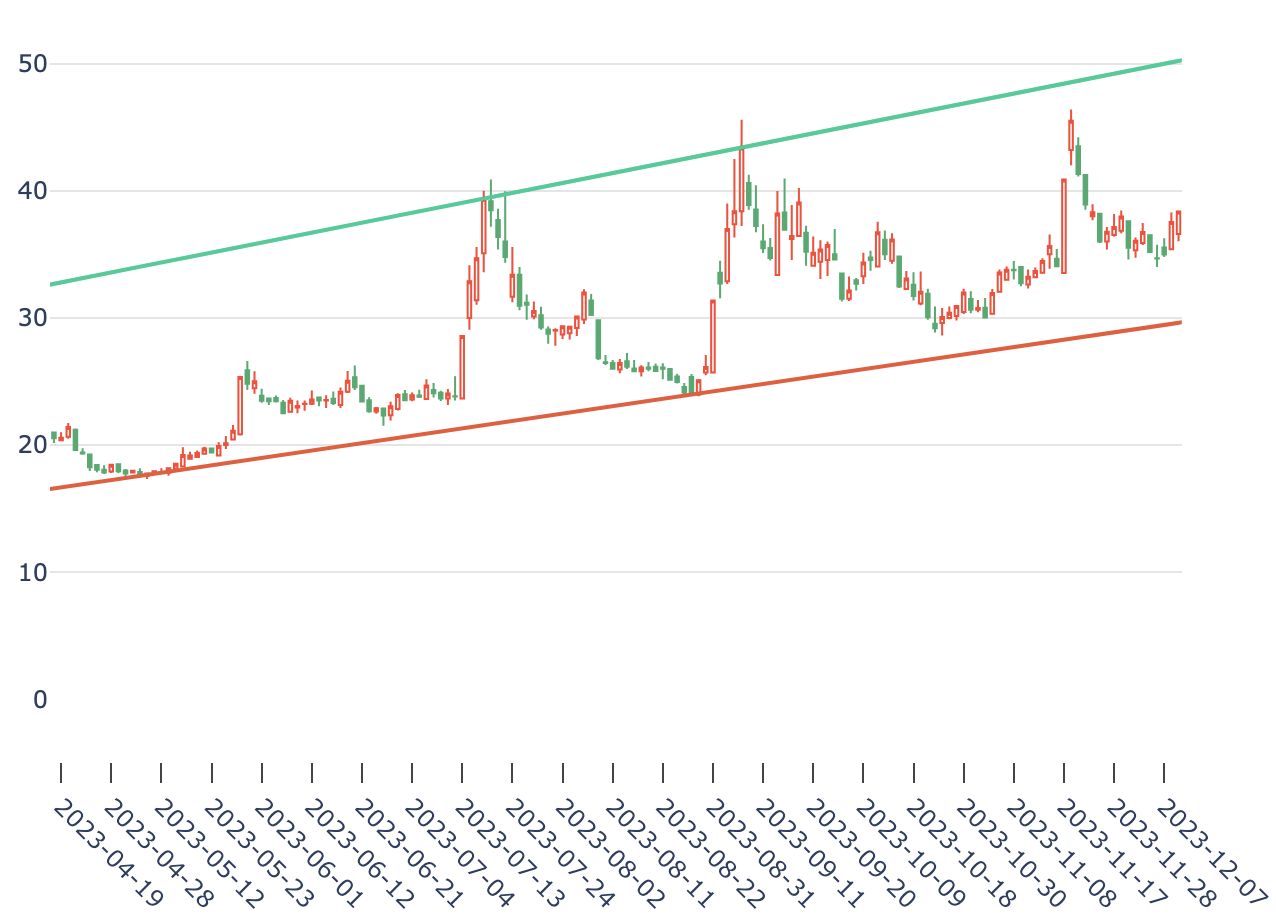
Since April 19, 2023, the asset has experienced four peaks. As time progresses, the consolidation pattern evolves.
On July 12, the pattern broke out as a divergent upward-biased triangle.
start = datetime.date(2022, 12, 1)
end = datetime.date(2023, 10, 29)
barss = load_bars(start, end, ("300814.XSHE", ))
for key, df in barss.groupby("asset"):
df = df.reset_index().set_index("date")
flag, resist, support = triangle_flag(df, datetime.date(2023, 7,19))
if flag != 0:
show_trendline(key, df, resist, support, flag, width=800, height=600)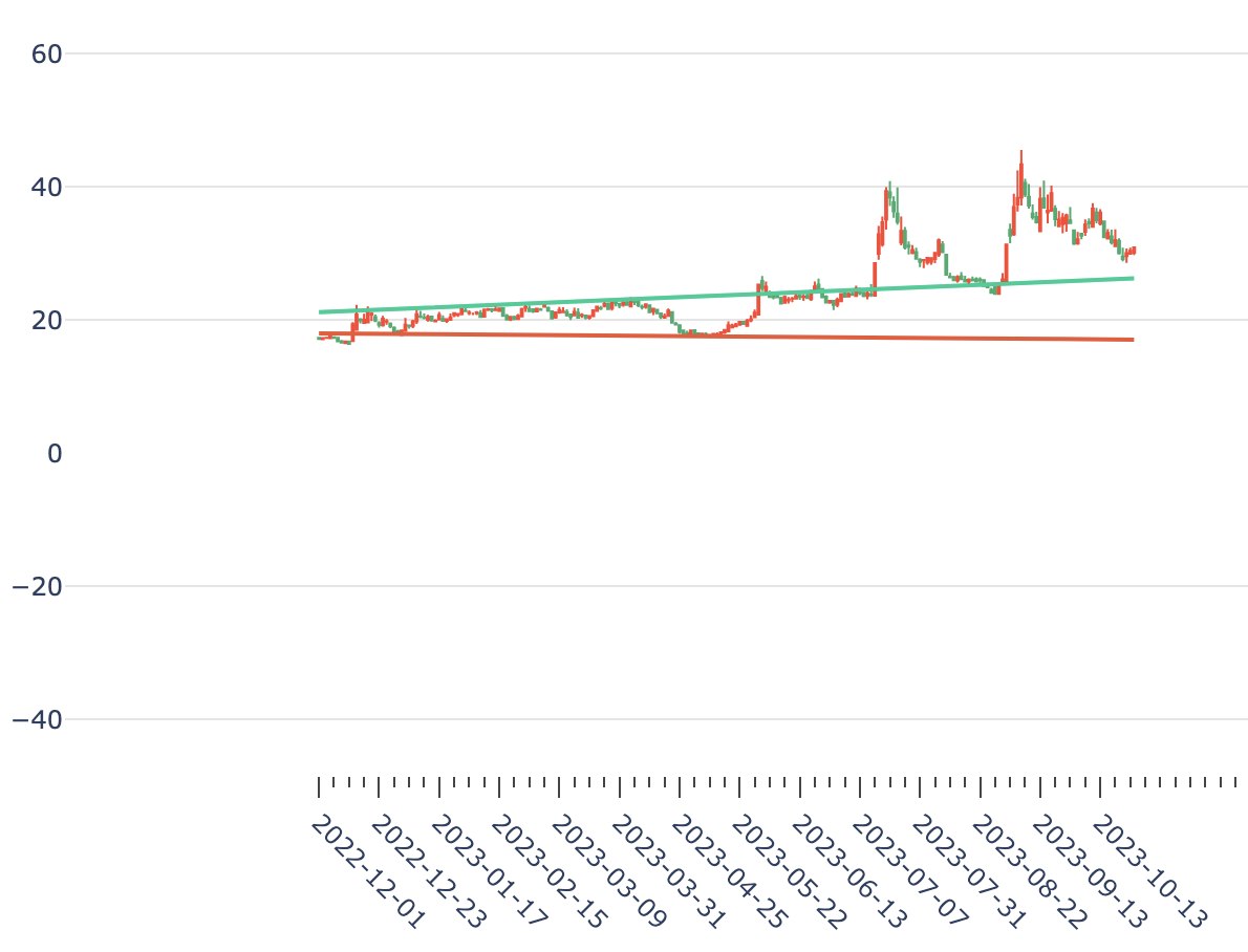
After the breakout on July 12, the support and resistance lines shifted. At this point, we could calculate the resistance level for September 7 to be 48 yuan. However, the price only reached 45.6 on that day, forming an upper shadow before closing.
start = datetime.date(2022, 12, 1)
end = datetime.date(2023, 10, 29)
barss = load_bars(start, end, ("300814.XSHE", ))
for key, df in barss.groupby("asset"):
df = df.reset_index().set_index("date")
flag, resist, support = triangle_flag(df, datetime.date(2023, 8,19))
if flag != 0:
show_trendline(key, df, resist, support, flag, width=800, height=600)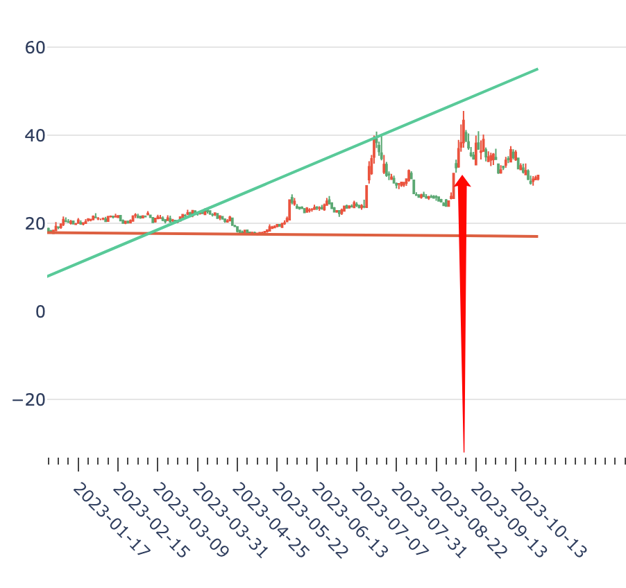
The pattern remained a rising triangle. However, after failing to break the resistance level on September 7, the resistance line should be recalculated using the two most recent peaks. The slope of this new resistance line is smaller than the previous one, indicating weaker subsequent momentum.
start = datetime.date(2022, 12, 1)
end = datetime.date(2023, 12,29)
barss = load_bars(start, end, ("300814.XSHE", ))
for key, df in barss.groupby("asset"):
df = df.reset_index().set_index("date")
flag, resist, support = triangle_flag(df, datetime.date(2023, 9,15))
if flag != 0:
show_trendline(key, df, resist, support, flag, width=800, height=600)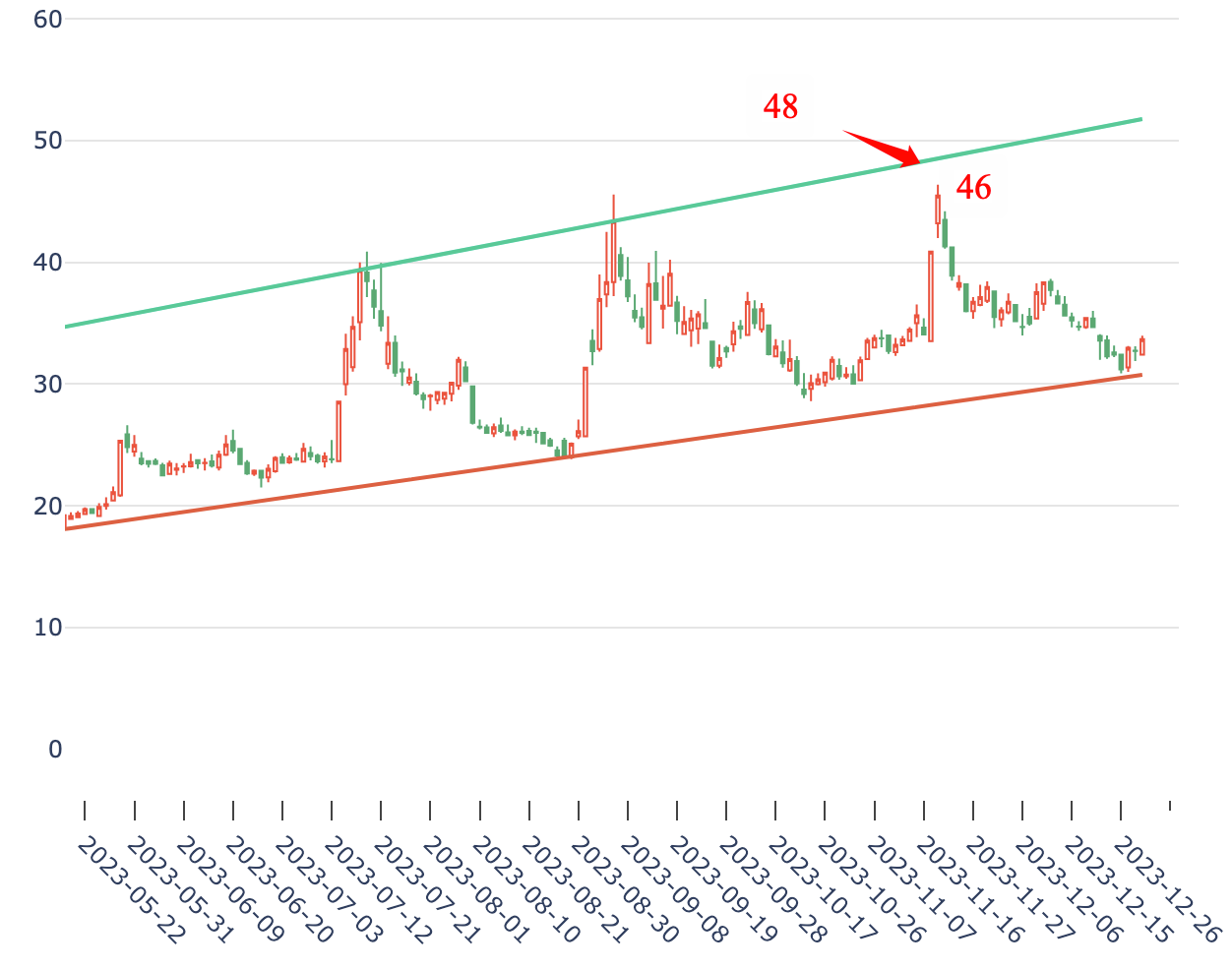
Following the new peak formation on September 7, the new resistance line projected a value of 48.5 on November 20. The actual high for that day was 46.4, again failing to break the resistance. Consequently, the resistance line must be recalculated. The slope of the new resistance line decreases further. The pattern transitions from a rising divergent triangle to a rising convergent triangle, signaling that it may be time to exit the position.
start = datetime.date(2022, 12, 1)
end = datetime.date(2023, 12,29)
barss = load_bars(start, end, ("300814.XSHE", ))
for key, df in barss.groupby("asset"):
df = df.reset_index().set_index("date")
flag, resist, support = triangle_flag(df)
if flag != 0:
show_trendline(key, df, resist, support, flag, width=800, height=600)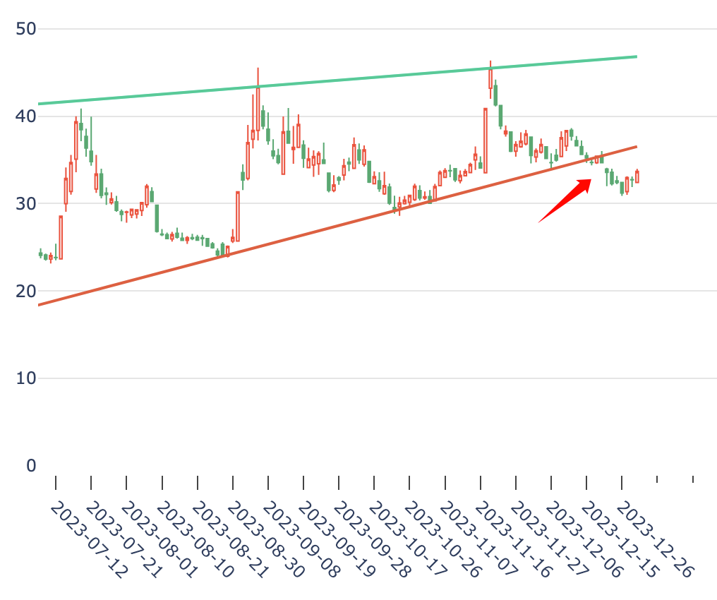
The changes in the slopes of these resistance lines help determine whether price increases are opening new channels or if momentum is expected to weaken, which is valuable for medium- to short-term trading strategies.
When constructing strategies using machine learning, we can use the changes in the slopes of the resistance and support lines ($\delta{S_r}$, $\delta{S_s}$) and the predicted values from these lines ($P_{t+1}$, $V_{t+1}$) as features. This approach allows for more precise predictions of future price movements.