
Why PE Fails as a Quant Factor: A Noise-Reduction Approach
In our September 16 WeChat Official Account article ("A Heart-Stopping Scene Before the Holiday! Who Can Tell Me If China A-Shares Are Undervalued?"), we highlighted a key data point: China A-shares' Price-to-Earnings (PE) ratio had reached a historical low, sitting at the 10th percentile. Just two days later, starting September 18, the Shanghai Composite Index (Shanghai Composite) embarked on a mini-bull run lasting two months.
When the Shanghai Composite climbed back to 3452, where does the current PE ratio stand? This is the first question we aim to answer today.
However, the primary focus of this article is to investigate the effectiveness of PE as a quantitative factor. We will propose a novel perspective and draw interesting conclusions for both individual stocks and the Shanghai Composite Index.
The PE Factor
In quantitative finance, PE is generally referred to as a valuation factor. It is a subcategory of value factors. Value factors include book-to-market ratio, profitability factors (ROE), investment factors, and others.
The formula for calculating PE is:
$$\text{PE} = \frac{\text{Stock Price}}{\text{Earnings Per Share}}$$
The conventional wisdom is that undervalued companies may see their stock prices rise, while overvalued companies may see their prices fall, thereby achieving a mean reversion of price to value.
In practice, however, using PE as a factor is fraught with pitfalls.
- The PE value relies on the financial metric of Earnings Per Share (EPS), which is reported quarterly. Therefore, between data releases, it only carries noise information such as closing prices (relative to the factor itself).
- Generally, factor analysis involves cross-sectional analysis—comparing and ranking the same attribute across different assets at the same point in time. However, the differences in an asset's PE are primarily determined by its industry, not the asset itself. Therefore, to calculate alpha using PE as a factor, you must perform sector neutralization.
- For cyclical industries, high PE values (or even negative values) often signal a buying opportunity, as company profits are expected to improve, allowing for profit-taking later. Conversely, low PE values signal a selling opportunity, as profits are expected to decline and bad news accumulates, forcing sellers to lower prices to offload shares.
But as they say, seeing is believing. Let's backtest it. When backtesting, we must use the PE_TTM metric rather than PE. PE_TTM stands for Trailing Twelve Months PE. PE is published on an annual basis, making its data response slow. PE_TTM, while still calculated on an annual basis, is computed and published over a rolling 4-quarter window, allowing it to reflect changes in company earnings more promptly.
start = datetime.date(2018, 1, 1)
end = datetime.date(2023, 12, 31)
universe = get_stock_list(start, code_only=True)
barss = load_bars(start, end, tuple(universe))
pe = get_daily_basic(["pe_ttm"], start, end, universe) * -1
prices = barss.price.unstack(level="asset")
merged = get_clean_factor_and_forward_returns(pe, prices)
create_returns_tear_sheet(merged)Here, get_daily_basic is our wrapper for the Tushare function, corresponding to Tushare's daily_basic function, but it allows fetching data for a specific indicator in one go.
Note line 6, where we multiply PE by -1. If you don't understand why, you might want to consider taking the course "Factor Analysis and Machine Learning Strategies."
This is the annualized Alpha from the backtest. On our WeChat Official Account, we have featured factors with annualized Alpha exceeding 15% multiple times—selected from countless failures. In reality, many factors are like PE:
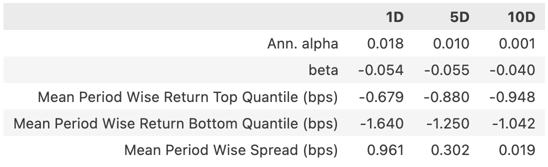 Annualized Alpha of PE Factor
The layered mean return chart also indicates that this factor does not have a strong linear relationship with returns.
After hitting a wall, let's step back and think about why.
First, PE is noisy data. In reality, over a one-year period with a sample of 250 data points, it only carries information 4 times. When we use PE as a factor, we are essentially using CLOSE as the factor.
Discovering Cyclical Trading Signals After Denoising
So, let's denoise PE. The method is to divide PE by the closing price. What we obtain is actually the reciprocal of Earnings Per Share.
The live pig industry is a strongly cyclical sector. Let's examine one example:
def deepinsight_fundamental(ticker: str, field, start, end, inverse = False):
df = get_daily_basic([field, "close"], start, end, (ticker,))
df = df.xs(ticker, level="asset")
if inverse:
df[field] = df["close"] / df[field]
else:
df[field] = df[field] / df["close"]
df["d1"] = df[field].diff()
df.ffill(inplace=True)
_, ax = plt.subplots(figsize=(15, 5))
ax.plot(df.index, df["d1"], label=f"{field}_denoise")
ax2 = ax.twinx()
ax2.plot(df.index, df["close"], label="close", color="r")
ax.legend(loc=2)
ax2.legend(loc=1)
plt.show()
start = datetime.date(2005, 1, 1)
end = datetime.date(2014, 10,31)
deepinsight_fundamental("002714.XSHE", "pe_ttm", start, end)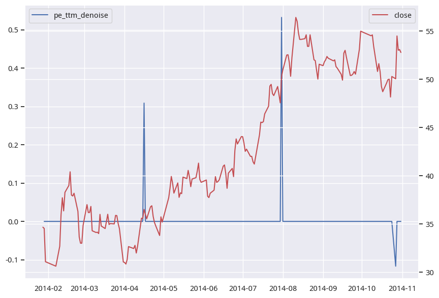 Cyclical Chart of a Live Pig Enterprise 2005-2014
This is the result from 2005 to 2014. We observe a clear signal around April 2014, after which the asset price rose by 60% (the actual rise is higher since Tushare data here is not adjusted for dividends/splits).
Let's look at the results from 2015 to 2022:
start = datetime.date(2014, 1, 1)
end = datetime.date(2022, 12, 31)
deepinsight_fundamental("002714.XSHE", "pe_ttm", start, end)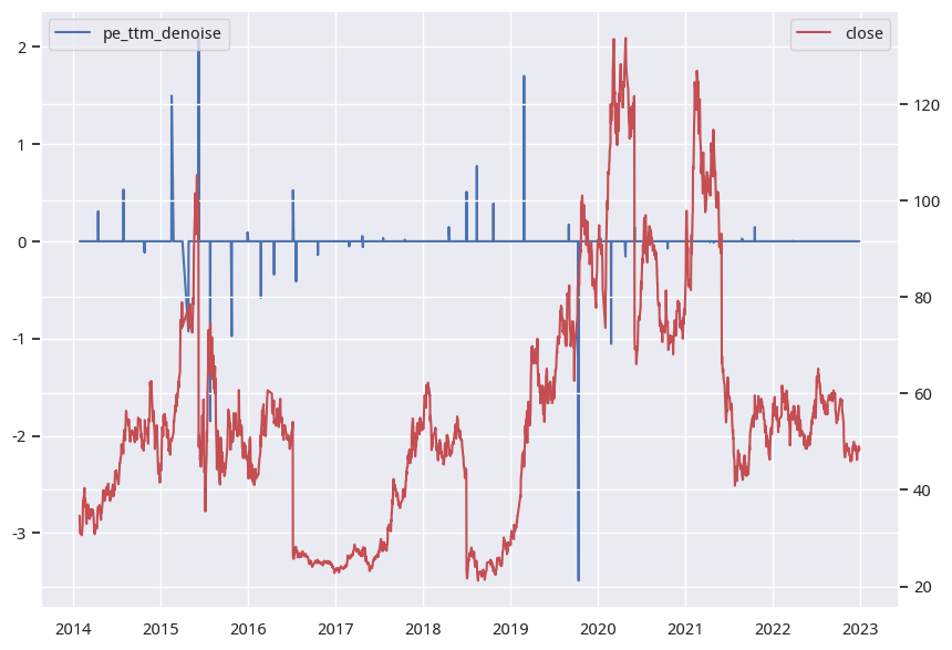 Cyclical Chart of a Live Pig Enterprise 2014-2022
Among a series of signals greater than zero, we focus on the first one, which marks the starting point for buying; among a series of signals less than zero, we also focus on the first one, which marks the starting point for selling (due to quarterly publication timing, there may be a slight lag).
In the chart above, we see a relatively clear buying opportunity around September 2018, followed by an increase of approximately 4 times, until a strong selling signal appeared in the third quarter of 2019 (the line below -3). A decline followed, lasting until early 2020. Although the stock price rose and fluctuated afterward, the signals were predominantly weak selling.
tip
This method is designed for strongly cyclical stocks. It is not suitable for weakly cyclical stocks.At 3450 Points, Is the Shanghai Composite Index High Now?
We always let the data speak. First, let's fetch the Shanghai Composite Index data:
import akshare as ak
pe = ak.stock_market_pe_lg(symbol="上证")
pe.set_index("日期", inplace=True)
pe.index.name = "date"
pe.rename(columns={"平均市盈率": "pe", "指数": "price"}, inplace=True)
pe.tail(15)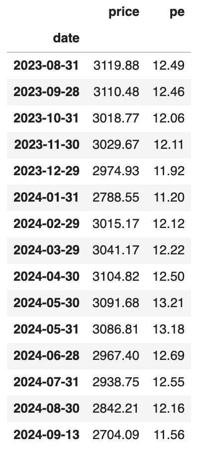
This gives us the complete PE data for the Shanghai Composite Index since 1999. We use the same method to examine the profitability of the entire market.
a = pe.copy()
a["adj"] = a.price/a.pe
a = a[["price", "adj"]]
a.plot(secondary_y='price', figsize=(15,5))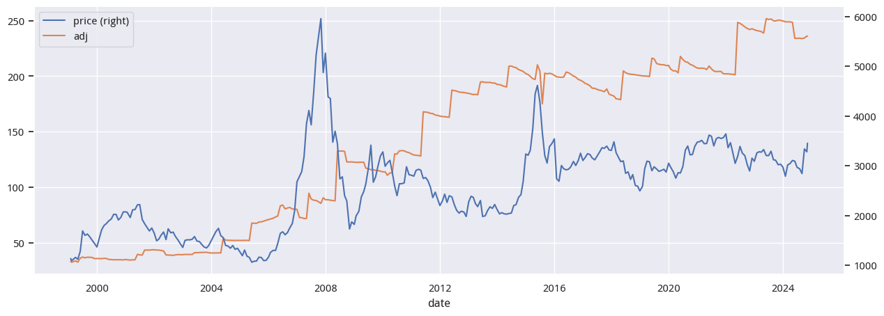 PE Trend After Denoising vs Index
From the chart, we can see that over the years, the profitability of China A-shares (hereinafter referred to as the indicator) has been rising. However, the speed of this rise has varied. Between 2004 and 2012, the rise was rapid, ultimately driving the index's mean reversion from decline to growth, though there was some overreaction at the high of 6000 points. After 2016, the indicator's trend flattened, and stock prices were affected accordingly, which explains the "eternal 3000 points" phenomenon.
From early 2016 to early 2024, this indicator rose by 25%. At that time, the index was at 2737 points; a 25% rise would bring it to around 3421 points. This is the broad trend—it is not precise, but rather a hypothesis.
Finally, let's answer where the Shanghai Composite Index at 3450 points stands in terms of percentile since 2016.
start = datetime.date(2016, 1, 1)
pe2016 = pe.loc[start:]
rank = pe2016.rank().loc[:, "pe"]
percentile = rank / len(pe2016)
percentile.plot()
p30 = 0.3
p70 = 0.7
# 30th and 70th Percentiles
plt.axhline(y=p30, color='green', linestyle='--', label='30th Percentile')
plt.axhline(y=p70, color='red', linestyle='--', label='70th Percentile')
# Get the last period's PE value and its date
last_pe = pe2016['pe'].iloc[-1]
last_date = pe2016.index[-1]
# Annotate the last period's PE value on the chart
plt.annotate(f'PE/Percentile: {last_pe:.2f}/{percentile.iloc[-1]:.1%}',
xy=(last_date, percentile.iloc[-1]),
xytext=(last_date, percentile.iloc[-1] + 0.05),
arrowprops=dict(facecolor='red', shrink=0.05))
# Add legend
plt.legend()
# Display the graph
plt.show()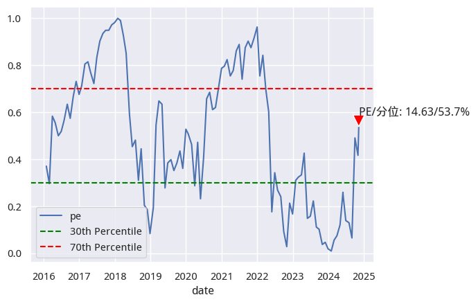
The data shows that the current position is at the 54th percentile since 2016. We are currently in a zone where we can both advance and defend, with no obvious indicator suppression and no offensive momentum provided. How to operate at this point is left to other indicators!