24-Lesson Quant Trading Course: From Data to Live Trading

This course comprises 400,000 words, 461 code snippets totaling over 7,000 lines (excluding bonus strategy code provided as a bonus), and offers a single-sentence summary: a course covering the entire quantitative trading workflow, enabling you to transition directly to live trading upon completion.

The curriculum is divided into six parts and 24 chapters. Below is an overview of the content for each part, reflecting our considerations in topic selection and course structuring:

Part 1: Where Does Data Come From?

Quantitative trading presupposes access to massive amounts of reliable data.

For institutional investors, the primary financial terminals used are Eastmoney Choice and Wind Information. Data providers include Wind, Hundsun Juyuan, Chaoyang Yongshu, Tianruan, Juchao, Tianxiang, Juling, Guotai An, and Tonglian. Chaoyang Yongshu holds advantages in analyst consensus expectations, earnings forecasts, and private equity data. Tianruan Technology excels in high-frequency market data. The Guotai An database is primarily for academic purposes, with comprehensive corporate finance data.

Individual and small-scale private equity investors mainly use data sources such as Tushare, AKShare, jqdatasdk, and QMT. These are the primary focus of this section.

This section consists of 5 lessons. We will focus on AKShare, Tushare, jqdatasdk, and Omicron—the data SDK built into the Daifuweng framework. We will also mention YFinance and other sources, clarifying which are viable and which are obsolete to save you time.

Saving you time is a key objective of this course. We believe that even without this course, you might piece together a quantitative tutorial yourself, but it would take much longer to find the right direction, causing you to lose first-mover advantage.

When introducing each data source, we cover its API style, documentation style, API categorization, and specifically how to retrieve trading calendars, security lists, and market data. Each source offers dozens or hundreds of APIs, so categorized introduction is crucial. Once you master the API style and documentation of each framework, exploration becomes effortless.

Considering it unreasonable to ask students to purchase data themselves (given the limitations of free data) while also needing data to demonstrate programs, we have built a quantitative environment providing real-time and historical market data (approximately 4 billion records) and a backtesting platform for your use. This is why we introduce Omicron—apologies for choosing this name in 2019; it went viral globally, but we did not.

Furthermore, this section lays the foundation for the entire series. We cover knowledge closely related to data processing, such as security code encoding, exchange codes, adjustment methods (forward/backward adjustment), and rounding issues in financial data processing. Here, we address seemingly simple yet often overlooked or unconsidered issues that are critical:

Is your usual rounding method correct?

You may never have thought about this. "Isn't it just math.round? How could it be wrong?" But you surely know the consequences of rounding errors: for low-priced stocks under 2 yuan, rounding can introduce an error of 0.01 yuan, equivalent to at least 0.5 percentage points!

This is not the only impact of rounding errors. In fact, it affects price granularity at the microstructure level, influencing the distribution of buy and sell orders. Interested readers, especially those in high-frequency trading, can refer to the paper Is Stock Price Rounded for Economic Reasons in the Chinese Markets to understand the special role of integer prices and auspicious numbers in A-share pricing, and similar patterns in global markets.

Now, let us tell you: Python’s implementation is indeed wrong!

Some quantitative tutorials suggest avoiding forward adjustment and using backward adjustment instead. We will ask you to rethink this. Once we reveal that forward and backward adjustment are merely linear transformations, you may think deeper: since linear transformations generate no new knowledge, what is the actual difference between forward and backward adjustment?

In this section, we also reveal the value of data. We explain how to obtain data such as investor counts and index PE ratios, and how they correlate with the Shanghai Composite Index’s movements, which is helpful for timing decisions over long cycles.

Some libraries are useful and well-written. But software is a technology full of regrets. We will also provide improvement suggestions for certain open-source software. If you are looking to contribute to open-source quantitative software, you might start with our suggestions to help完善 them.

Part 2: Introduction to Strategies

We use three lessons to introduce three strategies from three dimensions. Placing strategies in the second part serves two purposes: first, after completing the first part, some students may be eager to try; more importantly, these strategies demonstrate from different angles what skills are required to build a robust strategy, helping you understand why the subsequent course is structured this way.

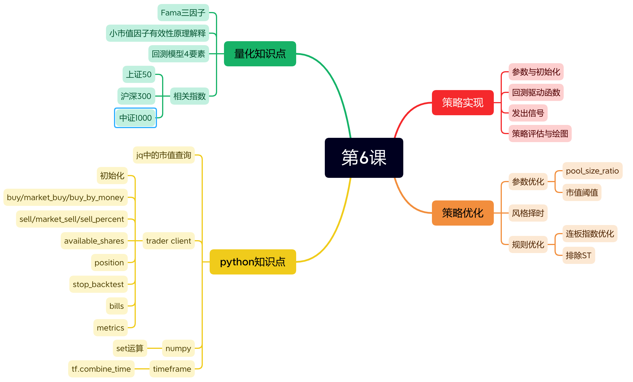
In Lesson 6, we introduce a small-cap strategy, which is a fundamental dimension. The small-cap factor is part of the Fama (FF) three-factor model. Its effectiveness has been validated by Wall Street for decades and was also highly effective in A-shares before 2017, entering a phase of intermittent effectiveness and失效 thereafter. This lesson answers several questions:

1. What minimum functionality must the simplest strategy implement?
2. After backtesting, how do we plot the asset curve and strategy metrics?
3. From which directions should we optimize the strategy?

The code in this lesson is short, direct, and easy to understand, with no tricks. However, we leave an assignment: how to abstract common parts of the strategy and backtest into a reusable framework?

Easy saying than done. Once you have manually implemented this, your understanding of quantitative trading will deepen. By Lesson 19, when we discuss complex backtesting frameworks like Backtrader, you should be able to get up to speed quickly and understand questions like:

Why does my strategy eat meat in backtests but dirt in live trading?

This is not necessarily your fault. Backtesting frameworks have their own choices and difficulties. Those who haven’t developed a backtesting framework don’t know this, nor could they tell you. But if you don’t understand the flaws of your weapons, how can you ensure they fire reliably on the battlefield?

In Lesson 7, we introduce the Bollinger Bands strategy. This is a technical analysis dimension. Bollinger Bands use only the simplest statistical theory—properties of the normal distribution. We rarely use it alone now, but as a single strategy, it once shone brightly, supporting a startup. Moreover, the principle of normal distribution is a cornerstone of statistical and financial data analysis.

Technical analysis (broadly defined as excluding fundamental analysis and macro-timing) is the most effective strategy method for medium and small-scale funds in A-shares. From the latest Huatai Securities Research report (August 2023), we see that the most effective factors in July were still reversal factors and volatility factors, with small-cap ranking third. This remains an era where technology reigns.

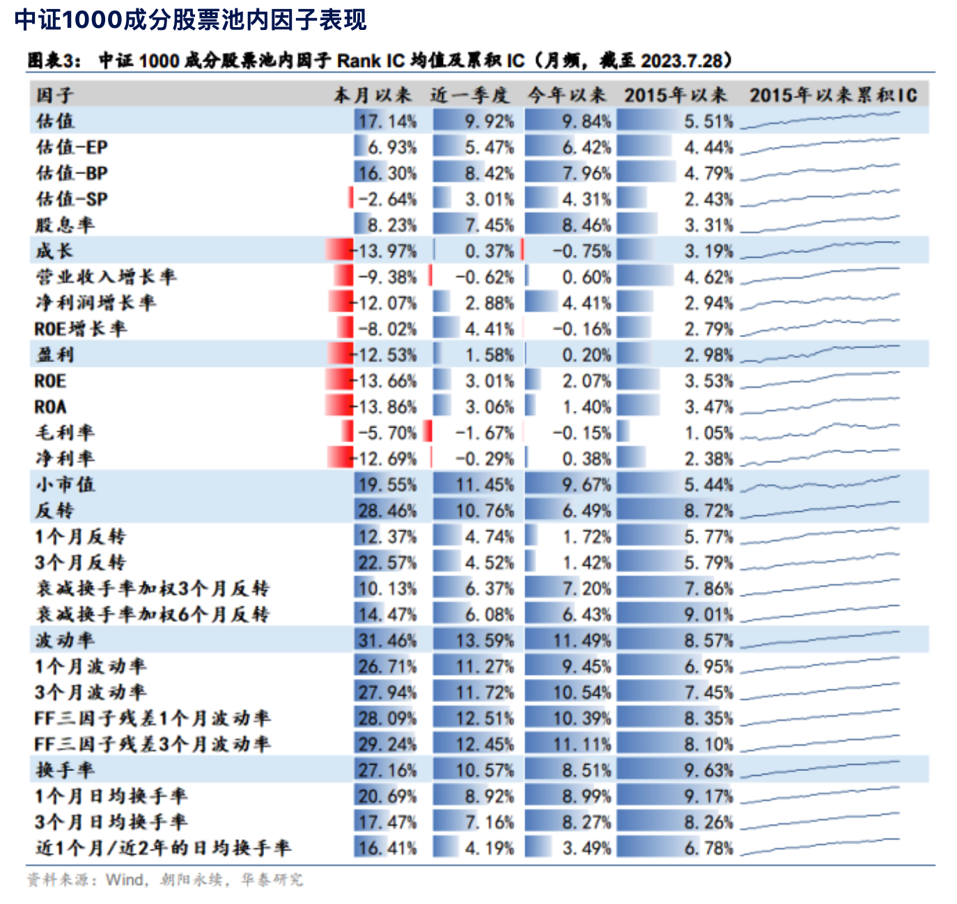
These factor performance data reveal the general direction of strategy research. You should have better methods to find reversals and master volatility. If you are interested in implementing these factors, you can find answers in our course Factor Analysis and Machine Learning Strategies.

In Lesson 8, we introduce grid trading, a strategy that doesn’t require a strategy, built from the trading dimension. It fully embodies the advantages of quantitative trading: avoiding emotional operations, strictly executing discipline, and potentially achieving profitability even without a complex strategy.

When you have a fishing net, the key is knowing where to cast it. The prerequisite for grid trading success is that the stock price ranges sideways for a long period. We indicate what conditions or targets are likely to result in long-term sideways movement. This includes conclusions based on behavioral finance principles and answers derived from trading rules. After completing the subsequent lessons, you will have the ability to programmatically identify such targets.

Part 3: Python Quantitative Trading Data Analysis

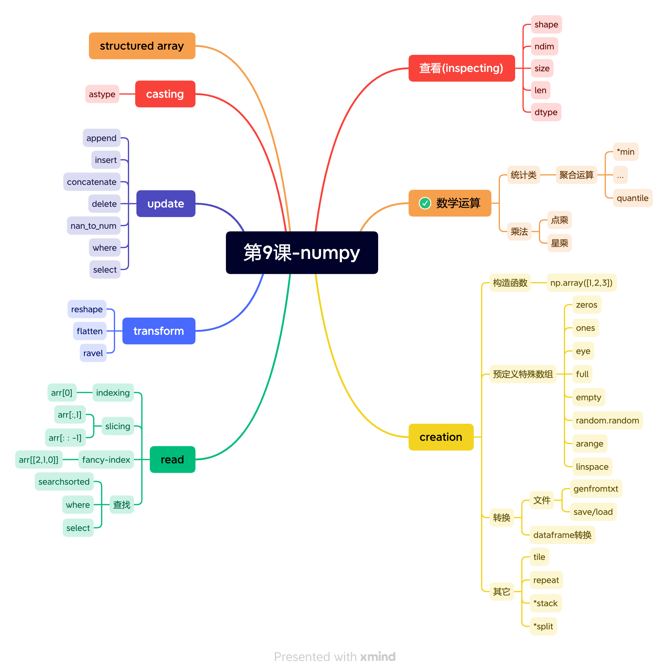
Lesson 9 introduces NumPy and Pandas, which are generally the basic data structures for quantitative trading, while we also have numerous operations requiring NumPy and Pandas.

Predicting price movements is difficult but possible in extreme cases. For example, if the Shanghai Composite Index has risen for 7 consecutive days, what is the probability of it rising or falling tomorrow? Predicting a drop would have a high probability of being correct. We set aside this probability calculation problem for now and return to the simplest question: how to programmatically detect if a security has experienced N consecutive days of gains?

Almost anyone who can code and has basic securities knowledge can implement this. But you need to do it better: for example, without loops, using only one line of code, and finding all N-day consecutive gains over the past few years at once. Speed is critical. Even if you trade only once a day, rebalancing before market close gives you only about two minutes (14:56 to 14:58) to traverse all market varieties (and perform strategy calculations). Your program must be fast; in practice, this is not easy.

In this lesson, we cover almost all high-frequency NumPy functions in common quantitative frameworks. The exercises in this section are also technical; mastering them will quickly make you a NumPy/Pandas expert!

In Lesson 10, we introduce TA-Lib, one of the most important technical analysis libraries, integrated into many quantitative frameworks.

In Lessons 11 and 12, we introduce some statistical knowledge. You will soon see its immense power!

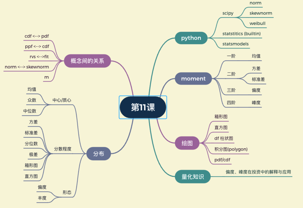
In these two lessons, we verify the fundamental question of what probability distribution the Shanghai Composite Index follows, and answer questions like "If the Shanghai Composite Index drops by 4%, should we buy the dip?" For more similar questions, we believe that after completing this course, you will naturally be able to explore and answer them.

Many people think probabilistic concepts are difficult to understand, such as PDF (Probability Density Function) / CDF (Cumulative Distribution Function). But we start with histograms, then imagine each bin size approaching zero, yielding the PDF. We believe that with this explanation, plus countless figures and code, probability and statistics are not so hard to understand?

Combining what we have learned previously, we can now perform some relatively difficult K-line pattern detection. This is the main content of Lesson 13—technical pattern analysis.

K-line pattern detection is very useful in a market dominated by retail investors; it is the basis for programmatically executing the Elliott Wave Theory. The essence of short-term trading is chip distribution; any rise or fall must fall into a limited number of paradigms. Therefore, K-line pattern detection, even if not used for prediction, can be used for post-hoc confirmation.

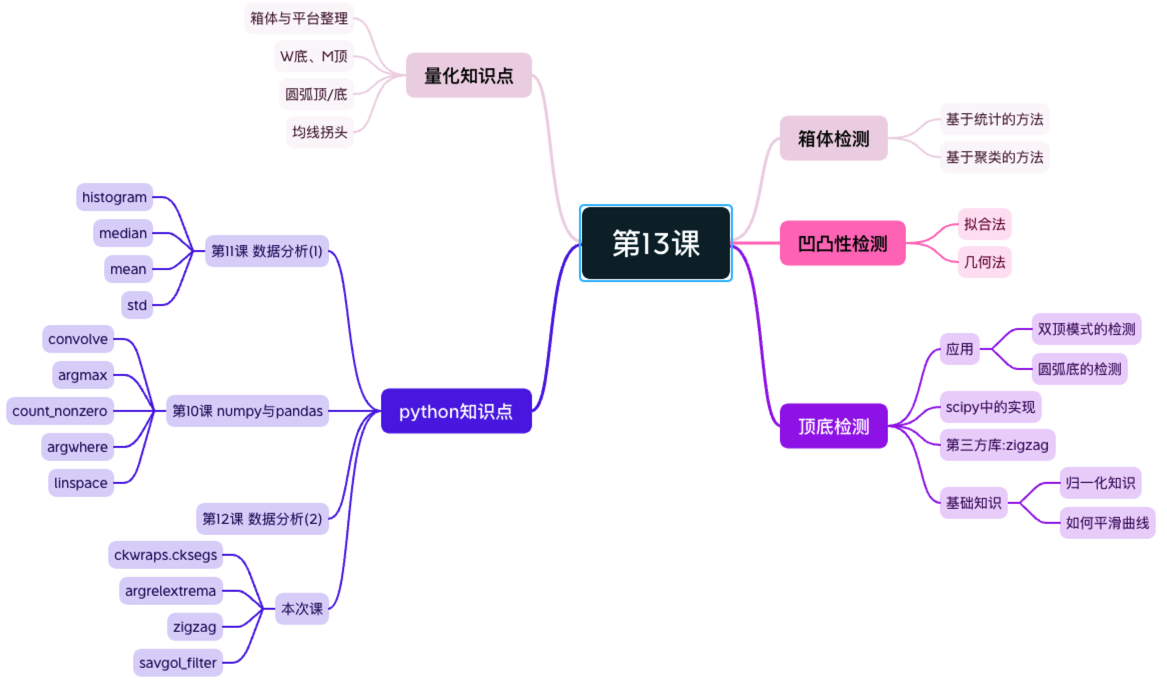
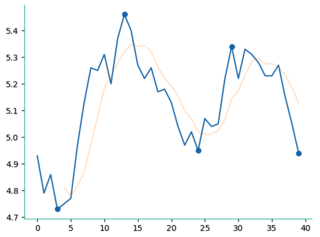
In this lesson, we provide a fully adaptive method for detecting tops and bottoms: based on probability distribution theory, with a solid mathematical foundation.

The red dots show the results of our adaptive algorithm detecting tops and bottoms. Based on these tops and bottoms, we calculated support and resistance lines. When the facts are laid before us, you have to admit that chartists sometimes indeed control the A-share market:

We can certainly use it for more things, such as detecting M-top and W-bottom patterns:

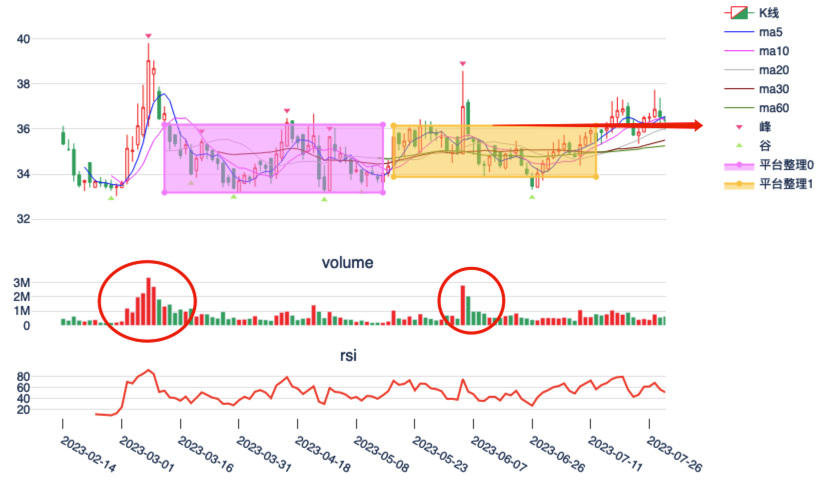
Or platform breakout detection (here we移植ed 2D clustering algorithms from machine learning to 1D time series):

And the principles and algorithms for intelligent RSI, etc.

If your goal in taking this course is to change jobs, then the content of Lesson 14—factor analysis—is indispensable. We detail all aspects of factor analysis: regression, IC, and layered backtesting, from principles to implementation.

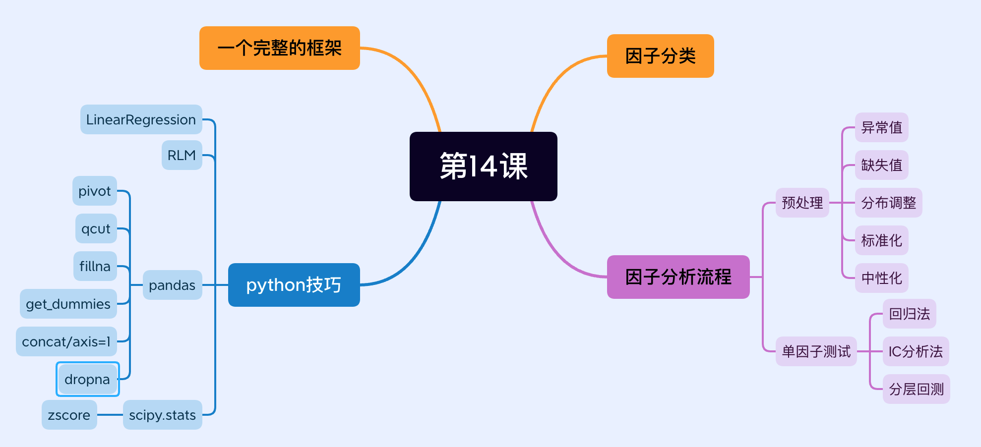
After completing the full process of factor analysis and having a panoramic view of most details and frameworks, Lesson 15 brings you to Alphalens. Now, learning Alphalens should be much easier, as you already know what it is and what it does.

Lessons 16 to 18 focus on visualization.

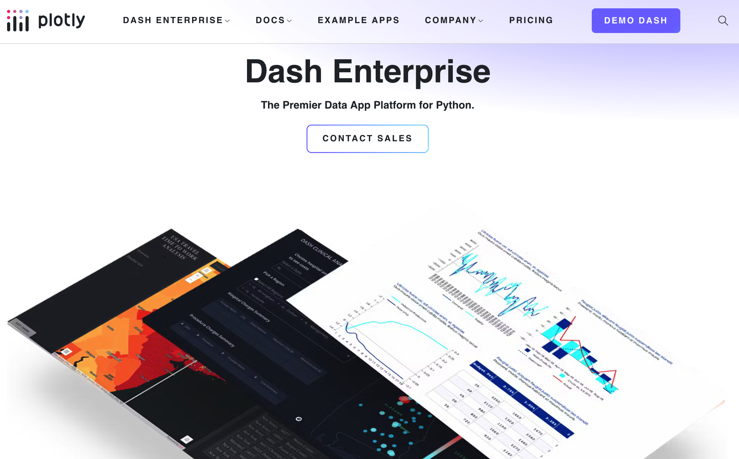
Plotting is not just for creating beautiful visualizations but also for unleashing the full potential of data and revealing hidden insights. It is the bridge between digital language and storytelling language, enabling individuals and organizations to make informed decisions and create meaningful change.

In quantitative trading, although we rely mainly on automated programs, we still rely on our intuition for factor exploration, generating backtest reports, and algorithm research. This intuition comes precisely from graphics.

In the course, we introduce superstars in the plotting world: Matplotlib, Plotly, Seaborn, and Pyecharts. Consistent with the course’s philosophy, we dissect the plotting frameworks and partially restore the mechanisms under the hood, ensuring you are never at a loss when facing new frameworks and new problems.

Part 5: Strategies and Backtesting

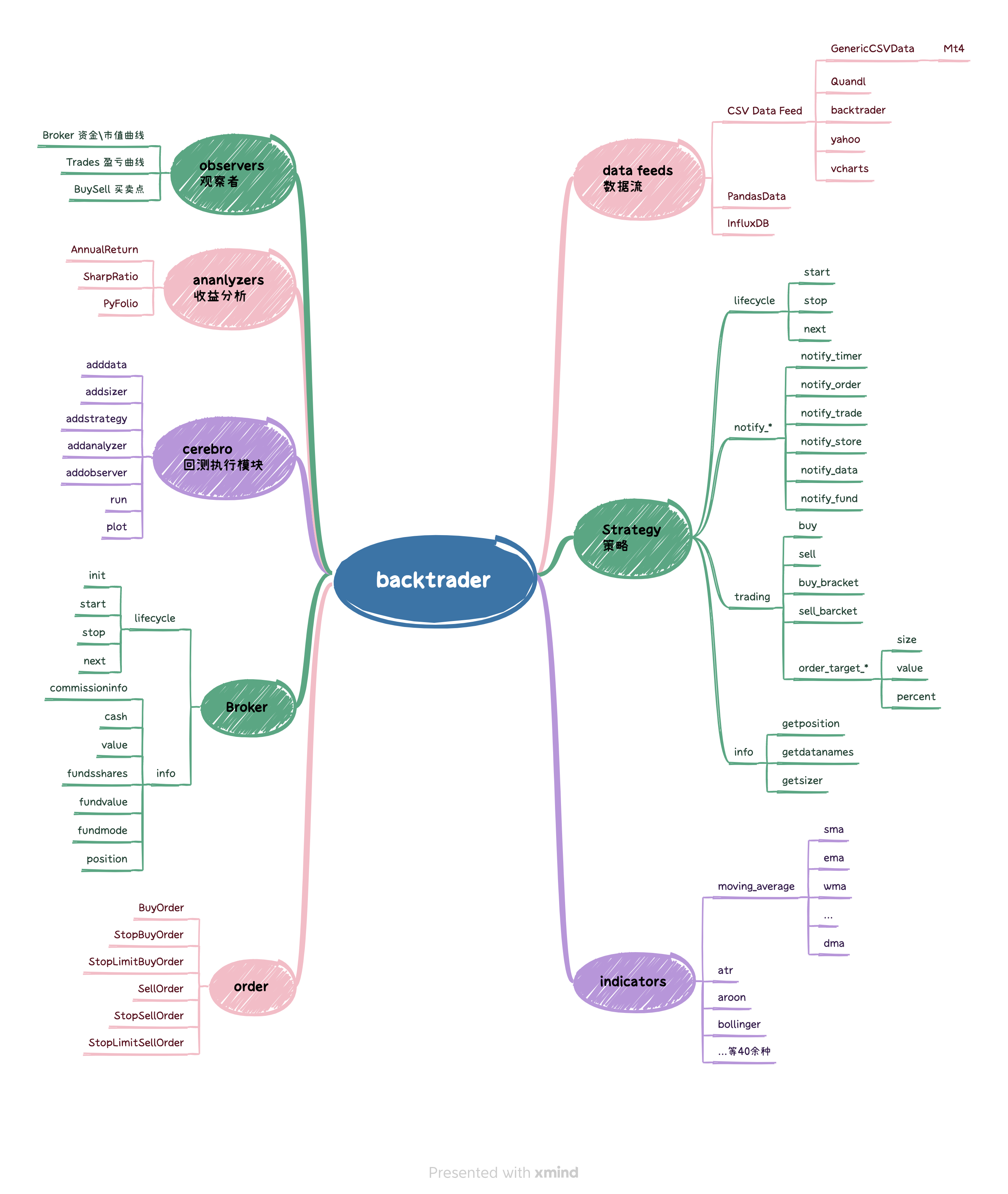
Lessons 19 and 20 introduce Backtrader, the most popular pure backtesting framework currently.

In Lesson 21, after becoming proficient in backtesting, we learn how to evaluate our strategies. We introduce the Sharpe ratio, Sortino ratio, annual return, and many other metrics, explaining how they reveal the balance between risk and profitability in a strategy. We also introduce a professional yet easy-to-use strategy evaluation metric plotting library—QuantStats.

Backtesting, like life, is full of traps. Some are brought by the framework itself—for example, some frameworks cannot use true adjustment (such as Backtrader; if you generate indicators all at once in __init__, regardless of the adjustment data used, you are using future data!); others stem from your strategy, calculation precision, misuse of look-ahead bias, dividends, trading rules, etc. We will detail these pitfalls in this lesson.

We will also introduce the Daifuweng backtesting framework. This is not to sell private goods, but because frameworks like Backtrader either cannot avoid the backtesting traps mentioned above, or require significant effort to modify. Considering that Daifuweng is open-source and its backtesting framework almost supports distributed backtesting—if I were to modify Backtrader, I might as well accept the Daifuweng backtesting framework. If your company is looking for a solution that complies with A-share trading rules, solves adjustment issues, and preferably has distributed infrastructure, we recommend studying this lesson carefully.

This is the content of Lesson 22.

Part 6: Connecting to Live Trading

Lessons 23 and 24 introduce how to connect to live trading. You will leave the rehearsal stage and enter live broadcasting from here.

We introduce EasyTrader, which has no capital threshold, and PTrade, QMT, and the quantitative trading platforms of Eastmoney and Huatai, which have certain capital thresholds. QMT is a quantitative platform launched by Xuntou. In addition to built-in strategy editing and backtesting functions, it provides a Python library named XtQuant, which we can use for its data and trading functions. Currently, QMT is the most cost-effective solution for connecting quantitative programs to live trading.

Ten years to sharpen a sword, the frosty blade has yet to be tested. After so many lessons of study and practice, I am convinced that you are ready to build your own money-printing machine!