
NumPy for Quant: Random Sampling, RNG, and IO
Random numbers and sampling are high-frequency operations in quantitative finance. Using NumPy’s random module, we can easily generate arrays of returns following a normal distribution, and calculate price trajectories via np.cumprod() to rapidly simulate an asset’s Sharpe ratio and price dynamics.
1. Random Numbers and Sampling
Random number generation and sampling are frequently used operations in quantitative finance, particularly useful for synthetic data creation. We have already used the normal() function in previous examples; it is a key function within the numpy.random module. By leveraging this function, we can generate price sequences that exhibit random volatility but trend upward, downward, or sideways overall.
tip
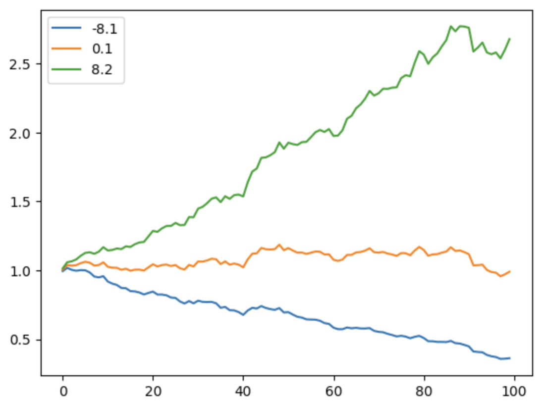
When do we need to synthesize price series? Beyond the examples mentioned earlier, consider this scenario: we want to understand the price trajectory of an asset with a Sharpe ratio of $S$, and how price dynamics relate to the Sharpe ratio. To answer this, we must use the "Monte Carlo" method to generate simulated data, calculate their Sharpe ratios, and plot them. Typically, we generate an array of returns following a normal distribution, weight them (to calculate the Sharpe ratio), and finally use the `np.cumprod()` function to compute the price trajectory for plotting.import numpy as np
from empyrical import sharpe_ratio
import matplotlib.pyplot as plt
returns_ = np.random.normal(0, 0.02, size=100)
legend = []
for alpha in (-0.01, 0, 0.01):
returns = returns_ + alpha
prices = np.cumprod(returns + 1)
sharpe = sharpe_ratio(returns)
_ = plt.plot(prices)
legend.append(f"{sharpe:.1f}")lines = plt.gca().lines
plt.legend(lines, legend)
From the plotted graph, we can see that when alpha is 1%, the Sharpe ratio reaches 8.2. Top-tier domestic fund managers can achieve a Sharpe ratio of approximately 2–3 within a year. You are encouraged to adjust the alpha parameter to observe its relationship with the Sharpe ratio.
1.1. The Legacy: np.random Module
Most tutorials on the web regarding NumPy random functions still use methods from the np.random module. Besides normal, the random package includes the following functions:
| Function | Description |
|---|---|
randint(a, b, shape) |
Generates a random integer array of shape shape within the interval $(a, b)$. |
rand(shape) |
Generates a random array of shape shape, filled with uniform distribution values from the interval $[0, 1)$. |
random(shape) |
Generates a random array of shape shape, filled with uniform distribution values. |
randn(d1, d2, ...) |
Generates a random array of shape shape, filled with normal distribution values. |
standard_normal(shape) |
Generates a random array of shape shape, filled with standard normal distribution values. |
| Function | Description |
|---|---|
normal(loc, scale, shape) |
Generates a random array of shape shape, filled with normal distribution values. loc is the mean, and scale is the standard deviation. |
choice(a, size, replace, p) |
Randomly samples size elements from a. If replace=True, repetition is allowed; otherwise, it is not. p represents probabilities; if p=None, each element is sampled with equal probability. |
shuffle(a) |
Randomly shuffles the elements in a. |
seed(seed) |
Sets the random number seed. If seed=None, the system time is used as the seed. |
As seen, NumPy often provides multiple methods for the same functionality. When memorizing these methods, first consider the distribution of the generated random numbers. The most basic distributions often have the simplest names: for instance, rand, randint, and random generate uniform distributions, while normal, standard_normal, and randn generate normal distributions.
Beyond uniform distributions, NumPy provides generation functions for many famous distributions, such as the F-distribution, Gamma distribution, Hypergeometric distribution, Beta distribution, Weibull distribution, and more.
Why does NumPy provide multiple functions within the same category? Some are provided for convenience to those who have used other well-known libraries (such as MATLAB).
randn is such an example; it is a function in MATLAB for generating normally distributed random numbers, now ported to NumPy. Another function we see here, rand, follows the same logic. In contrast, random is defined according to NumPy’s own API style.
The choice method has specific applications in quantitative finance. For example, we might want to randomly sample 10 stocks from a large universe for a small-scale trial, and then decide whether to sample more stocks based on the results.
The seed function sets the seed for the random number generator. It is very useful during unit testing or demonstrations (both cases require generating the same sequence of random numbers consistently).
1.2. New Style: default_rng
In the previous section, we introduced some random number generation functions but did not explain their underlying principles. The random numbers generated by NumPy are pseudo-random numbers, produced by a Random Number Generator (RNG). The output of an RNG is random, but identical inputs always produce identical outputs. Every method we call is essentially a sampling action on this sequence (based on the input size/shape).
In the numpy.random module, there exists a global RNG. When we call specific random functions, we are actually generating random numbers through this global RNG. This global RNG is often initialized by someone calling the seed method on it. This can cause issues because you may not know when, where, or with which parameter someone else has reset the seed.
For this reason, it is no longer recommended to directly use the methods in the numpy.random module. A better approach is to create an independent RNG for each specific application and call the corresponding methods on that object:
rng = np.random.default_rng(seed=123)
rng.random(size=10)rng is a RandomGenerator object. When initializing it, we need to pass in a seed. If omitted, NumPy will use the system time as the seed.
rng possesses most of the methods mentioned in the previous section, such as normal, f, gamma, etc.; however, methods ported from MATLAB no longer appear on this object. Additionally, randint is replaced by rng.integers.
Furthermore, the random number generator object produced by default_rng uses the PCG64 algorithm. Compared to the algorithm used in previous versions, it not only returns statistically better random numbers but is also 4 times faster.
warning
NumPy also contains a `RandomState` class. It uses the slower Mersenne Twister to generate pseudo-random numbers. This class is now deprecated and no longer recommended.We have introduced the functionality of choice. Now, let us look at an example of how to use choice to balance a dataset.
In supervised learning, we often encounter imbalanced data. For instance, we may want to train a classifier, but the class distribution in the training set is uneven. We can use the choice method to perform under-sampling or over-sampling on the dataset to address this issue.
For clarity, let us first generate an imbalanced training dataset. This dataset has three columns, where the first two are features (which you can imagine as factor exposures) and the third is the label.
import pandas as pd
import numpy as np
rng = np.random.default_rng(seed=42)
x = rng.random((10,3))
x[:,-1] = rng.choice([0,1], len(x), p=[0.2, 0.8])We visualize this dataset using the following method to verify that it is indeed imbalanced.
df = pd.DataFrame(x, columns=['factor1', 'factor2', 'label'])
df.label.value_counts().plot(kind='bar')The output is:
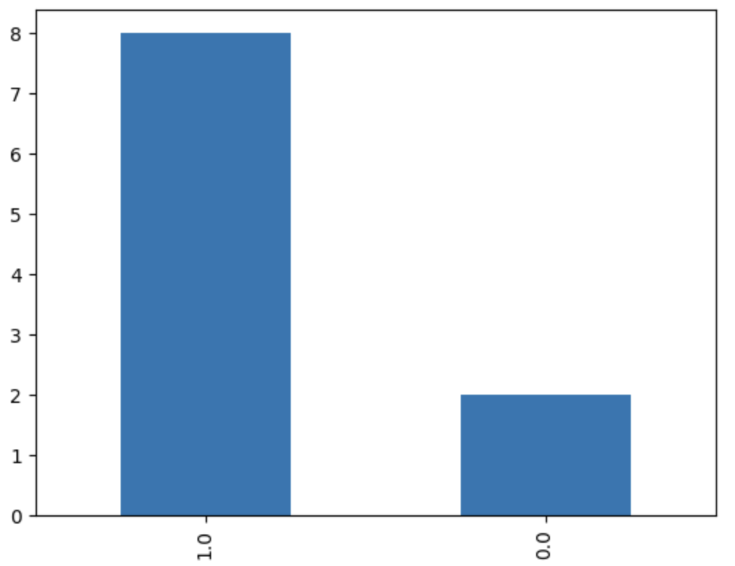
To obtain a new balanced dataset from this, we have two approaches: under-sampling, which involves sampling part of the majority class data so that its count equals that of the minority class; and over-sampling, which involves copying part of the minority class data so that its count equals that of the majority class.
The following example demonstrates how to perform under-sampling:
labels, counts = np.unique(x[:,-1], return_counts=True)# 最小分类的标签
min_label = labels[np.argmin(counts)]
# 最小分类样本的数量,作为 UNDER SAMPLING 的样本数量
min_label_count = np.min(counts)
# 最小分类无须抽取,全部提取
results = [
x[x[:,-1] == min_label]
]
# 对其它分类标签进行遍历,需要先剔除最小分类
for label in np.delete(labels, np.argmin(counts)):
sampled = rng.choice(x[x[:,-1]== label], min_label_count)
results.append(sampled)
np.concatenate(results)This code first identifies the minority class and its count, then iterates through each label, using rng.choice to randomly sample the minority class count for other classes, and finally concatenates all subsets.
This sample code can handle multiple labels. To perform over-sampling, simply replace min with max.
2. I/O Operations
We rarely use NumPy directly to read and write files. Improving I/O performance has never been NumPy’s primary focus, so a basic understanding suffices.
2.1. Reading and Writing CSV Files
NumPy can read data from CSV-formatted text files, primarily using the following methods:
| API | Description |
|---|---|
loadtxt |
Parses tabular data in text format. |
savetxt |
Saves data to a text file. |
genfromtxt |
Same as above, but allows missing values, providing advanced usage. |
recfromtxt |
A shortcut for genfromtxt, automatically inferring record arrays. |
recfromcsv |
Same as above; no need to specify the delimiter if it is a comma. |
Let us briefly demonstrate their usage with the following example:
import io
import numpy
buffer = io.StringIO("""1,2""")
# 默认情况下,LOADTXT 只能读取浮点数
numpy.loadtxt(buffer, delimiter=",")This outputs the array array([1., 2.]).
buffer = io.StringIO("""1,2,hello""")
# 通过指定 DTYPE 参数,可以读取其它类型
numpy.loadtxt(buffer, delimiter=",", dtype=[("age", "i4"), ("score", "f4"), ("name", "U8")])This yields a Structured Array, where the third column is of string type. If we do not specify the dtype parameter, loadtxt will fail to parse.
buffer = io.StringIO("""
1,2,hello
""")
numpy.genfromtxt(buffer, delimiter=",")Here, we use genfromtxt to load the data without specifying the dtype parameter. genfromtxt will parse non-numeric columns as nan. Therefore, this code outputs: array([1., 2., nan]).
Now, let us add the dtype parameter to genfromtxt:
buffer = io.StringIO("""1,2,hello""")
numpy.genfromtxt(buffer, delimiter=",", dtype=[("age", "i4"), ("score", "f4"), ("name", "U8")])The result we obtain is: array((1, 2., 'hello'), dtype=[('age', '<i4'), ('score', '<f4'), ('name', '<U8')]). Note that it is a Structured Array.
recfromtxt does not require dtype; it automatically infers the data type.
buffer = io.StringIO("""1,2,hello""")
numpy.recfromtxt(buffer,delimiter=",")This code outputs rec.array((1, 2, b'hello'), dtype=[('f0', '<i8'), ('f1', '<i8'), ('f2', 'S5')]). If the inference is inaccurate, we can manually add the dtype parameter.
If we use recfromcsv, we can even omit the delimiter parameter.
buffer = io.StringIO("""age,score,name1,2,hello""")
numpy.recfromcsv(buffer)The output is the same as the previous example.
For speed considerations, we can also use other libraries to parse CSV files and then convert them into NumPy arrays. For example:
# 利用 CSV.READER() 来解析,比 NUMPY 快 8 倍
np.asarray(list(csv.reader()))
# 利用 PANDAS 来解析,比 NUMPY 快 22 倍
pd.read_csv(buffer).to_records()2.2. Reading and Writing Binary Files
If we do not need to exchange data with external systems and the data is self-contained, we can also save data as binary files.
Use the numpy.save function to save a single array as a binary file, and the numpy.load function to read data saved by numpy.save. Files saved in this manner have the .npy extension.
To save multiple arrays, use the savez command. Files saved in this manner have the .npz extension. For more complex requirements, libraries such as HDF5 or PyArrow can be used to save data.