
NumPy Masked Arrays & ufuncs: Vectorized Quant Finance
“Masked Array is a critical NumPy concept that allows us to perform computations while masking invalid values, preserving data integrity. Meanwhile, ufuncs leverage low-level C implementations for vectorized operations, making complex calculations efficient and concise.”
1. Masked Array
You may often encounter NumPy masked arrays in low-level libraries. Masked Array is a significant concept in NumPy. Consider this scenario: you have a dataset containing missing data or invalid values. These “unqualified” data points might be represented as np.nan, np.inf, None, or other syntactically valid but semantically incorrect values (e.g., negative case counts in a COVID-19 dataset). How can we perform computations on this data while maintaining its integrity?
note
Here is a real-world example. You can find a COVID-19 dataset on [Kaggle](https://www.kaggle.com/datasets/atilamadai/covid19) that includes instances of negative cumulative case counts. This dataset was collected and provided by Johns Hopkins University.x = np.array([1, 2, 3, np.inf, np.nan, None])
np.mean(x)
np.nanmean(x)NumPy functions cannot process data containing np.nan, np.inf, or None. Even if the data is syntactically valid, forcing calculations on semantically invalid data yields incorrect results.
Here is a realistic scenario in quantitative finance: a company reports zero annual profit, making its Year-over-Year (YoY) profit growth impossible to calculate in the following year. If we need to use YoY data for further computations, we must mask this invalid year’s value. Otherwise, we won’t even be able to calculate the mean YoY profit.
A workaround is to copy the original data and replace invalid values with np.nan. Most operations can then be performed using np.nan* functions, which we have discussed previously. However, if you are the original data collector, you should obviously publish the data as-is; any modification would be inappropriate. If you are the data user, you should preprocess the data before computation. Yet, you might lack the necessary information to preprocess the data—how could you anticipate that seemingly harmless values like -1 or 0 are actually hidden errors?
To address this, NumPy provides Masked Array. However, we won’t dwell on it extensively. Regarding Masked Array, we can borrow this saying: Most people don’t need to know about Masked Array; those who do already master it.
One important note: use Masked Array only when necessary. Contrary to what you might imagine, Masked Array does not improve performance; in fact, it significantly degrades it:
import numpy as np
# NUMPY VERSION 1.24.4
g = np.random.random((5000,5000))
indx = np.random.randint(0,4999,(500,2))
g_nan = g.copy()
g_nan[indx] = np.nan
mask = np.full((5000,5000),False,dtype=bool)mask[indx] = True
g_mask = np.ma.array(g,mask=mask)
%timeit (g_mask + g_mask)**2
# 901 MS ± 52.3 MS PER LOOP ...
%timeit (g_nan + g_nan)**2
# 109 MS ± 72.2 ΜS PER LOOP ...As shown, Masked Array is nearly 9 times slower.
tip
If you must perform operations on arrays containing `np.nan`, try using the `nan*` functions from the `bottleneck` library. Since there is no `nansquare` function, but variance calculations inevitably involve squaring, we can evaluate the performance difference between NumPy and `bottleneck` using the `nanvar` function. %timeit np.var(g_mask)
# 587 MS ± 37.9 MS PER LOOP ...
%timeit np.nanvar(g_nan)
# 281 MS ± 1.46 MS PER ...
%timeit nanvar(g_nan)
# 61 MS ± 362 ΜS PER LOOP ...bottleneck is nearly 5 times faster than NumPy. If you are using an older version of NumPy, bottleneck will be even faster.
2. ufunc
ufunc is a crucial NumPy concept that performs element-wise operations on two input arrays simultaneously (e.g., addition, comparison). NumPy defines approximately 61 ufuncs. These operations are implemented in low-level C and support vectorization, making them generally faster.
For example, in NumPy, there are two similar functions to find the maximum value in an array: np.max and np.maximum. The latter is a ufunc, while the former is not. Apart from usage differences, the latter is faster.
arr = np.random.normal(size=(1_000_000,))
%timeit np.max(arr)
# 801 MS ± 54.7 MS PER LOOP ...
%timeit np.maximum.reduce(arr)
# 775 MS ± 12.1 MS PER LOOP ...np.maximum, as a ufunc, is designed to accept two arguments and cannot be used directly to find the maximum value of a one-dimensional array. In such cases, we must use the reduce operation to achieve the desired result.
Here, np.maximum is a ufunc, and reduce is one of the attributes of the ufunc object (in Python, everything is an object, including functions). Other attributes of ufunc include accumulate, outer, and reduceat.
accumulate is another commonly used attribute in ufuncs, which you may have encountered before. For instance, it is used when calculating maximum drawdown:
# 模拟一个股价序列
n = 1000
xs = np.random.randn(n).cumsum()
# 最大回撤结束期
i = np.argmax(np.maximum.accumulate(xs) - xs)
# 最大回撤开始期
j = np.argmax(xs[:i])
# 最大回撤
mdd = (xs[j] - xs[i])/xs[j]
plt.plot(xs)
plt.plot([i, j], [xs[i], xs[j]], 'o', color='Red', markersize=10)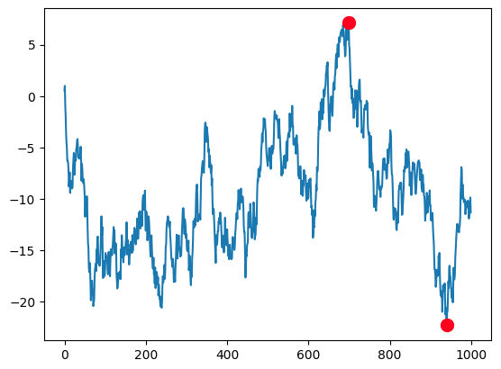
Simplicity is beauty. After using accumulate, we find that calculating maximum drawdown is as simple as just two or three lines of code.
ufuncs are so useful that you might wonder why you don’t use them more often. In fact, you likely use ufunc every day. Many binary mathematical operations are wrappers around ufuncs. For example, when we call A + B, we are actually calling the np.add(A, B) ufunc. They are equivalent in both functionality and performance. Other ufuncs include logical and comparison operations. If an operation accepts two arrays as arguments, NumPy has likely already implemented the corresponding ufunc. Additionally, some trigonometric functions, despite accepting only one array argument, are also ufuncs.
Therefore, the ufunc functions we need to pay special attention to and learn are mainly maximum, minimum, etc. Here is another common example in a quantitative scenario using maximum—calculating the length of the upper shadow.
tip
**Long upper shadows** are traces left after an asset’s failed upward attack. They are helpful for analyzing subsequent stock price movements. First, capital attacked this price level, revealing its intentions. Second, the attack failed, often leading to a washout (or collapse) next. Long upper shadows at the bottom of the stock price are also called “Immortal Guiding Finger” by experienced traders, indicating a higher probability of a subsequent rally. When upper shadows appear at high levels, they are likely top-signaling signals. At this point, on lower-level K-lines, obvious top-signaling signals such as moving average turns may already have appeared.$$ upper_shadow = high - max(open, close) $$
The figure below also shows the upper shadow:
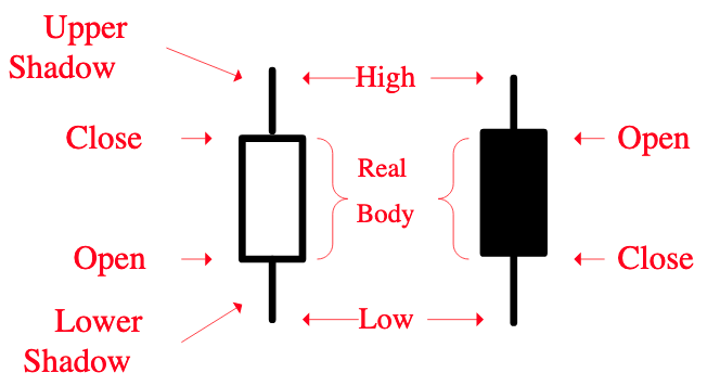
If upper_shadow > threshold, a long upper shadow can be considered present (of course, upper_shadow needs to be normalized). Detecting a single day’s upper shadow is simple. The following code demonstrates how to solve this vectorially:
import numpy as np
import pandas as pd
rng = np.random.default_rng(seed=78)
matrix = rng.uniform(0.98, 1.02, (4, 30)).cumprod(axis=1)
opn = matrix[0]
close = matrix[-1]
high = np.max(matrix, axis=0)
upper_shadow = (high - np.maximum(opn, close))/close
np.round(upper_shadow, 2)The code on line 10 consists entirely of ufuncs. Here, we use np.subtract (subtraction), np.maximum, and np.divide (division). maximum compares elements from two equally long arrays, opn and close, element-wise, and takes the larger one to form a new array, which is also of the same length as opn and close.
To calculate the lower shadow length, you can use minimum.
Copyright Notice
All materials for this course, including all text, images, code, and exercises, are developed by the author, except where cited. All draft versions are managed through third-party git services as proof of copyright. Please do not cite without written authorization from the author.
During the writing of this article, a small amount of code and text referenced content generated by Tongyi Lingma.