
Numpy Vectorization in Quant: Outlier Clipping, Rolling MDD, and Adaptive Signals
Outlier clipping is an indispensable step in quantitative analysis preprocessing. Among various methods, the median pullback approach is widely adopted for its robustness and adaptability. By leveraging Numpy’s vectorized implementation, we can easily perform multi-asset outlier clipping, significantly boosting computational efficiency.
Another Example of Vectorization: Multi-Asset Median-Based Outlier Clipping
Outlier clipping is a common step in quantitative analysis preprocessing and is also prevalent in machine learning. Among various outlier clipping methods, median pullback is the most robust and adaptable to different data distribution characteristics.
First, let’s introduce the concept of Median Absolute Deviation (MAD):
$$MAD = median(|X_i - median(X)|)$$
To use MAD as an estimator consistent with the standard deviation $\sigma$, we define: $$\hat{\sigma} = k \cdot MAD$$
Here, $k$ is a proportionality constant. If the distribution is normal, we can calculate: $$ k = \frac{1}{\Phi^{-1}(\frac{3}{4})} \approx 1.4826 $$
Based on this $k$ value, taking 3 times MAD approximates to 5 times the standard deviation.
The code implementation is as follows:
from numpy.typing import ArrayLike
def mad_clip(arr: ArrayLike, k: int = 3):
med = np.median(arr)
mad = np.median(np.abs(arr - med))
return np.clip(arr, med - k * mad, med + k * mad)np.random.seed(78)
arr = np.append(np.random.randint(1, 4, 20), [15, -10])
mad_clip(arr, 3)This code only performs mad_clip on a single asset. If we need to perform outlier clipping on a specific metric for all China A-shares simultaneously, the above method would require looping over 5,000 times, which is obviously slow. In this case, we can use the following method:
def mad_clip(df: Union[NDArray, pd.DataFrame], k: int = 3, axis=1):
"""使用 MAD 3 倍截断法去极值"""
med = np.median(df, axis=axis).reshape(df.shape[0], -1)
mad = np.median(np.abs(df - med), axis=axis)
magic = 1.4826
offset = k * magic * mad
med = med.flatten()
return np.clip(df.T, med - offset, med + offset).TThis version of mad_clip accepts both numpy ndarray and pandas dataframe as parameters. It returns data in the same format as the input.
We passed the axis parameter in the np.median call. If axis=0, it indicates traversal along the column direction, meaning we take the median across rows (i.e., across assets for each date). If axis=1, it indicates traversal along the row direction, meaning we take the median across columns (i.e., across dates for each asset).
Let’s test this with real data:
# 加载测试数据
start = datetime.date(2023, 1, 1)
end = datetime.date(2023, 12, 29)
barss = load_bars(start, end, 7)
closes = barss["close"].unstack("asset").iloc[-5:]
closesThe output data is:
| asset/date | 002095.XSHE | 003042.XSHE | 300099.XSHE | 301060.XSHE | 601689.XSHG | 603255.XSHG | 688669.XSHG |
|---|---|---|---|---|---|---|---|
| 2023-12-25 | 23.400000 | 18.090000 | 6.10 | 13.00 | 73.910004 | 36.799999 | 18.080000 |
| 2023-12-26 | 21.059999 | 17.520000 | 5.94 | 12.83 | 72.879997 | 37.000000 | 18.080000 |
| 2023-12-27 | 20.070000 | 17.590000 | 6.04 | 12.84 | 72.000000 | 36.840000 | 18.049999 |
| 2023-12-28 | 20.010000 | 18.139999 | 6.11 | 13.14 | 72.199997 | 38.150002 | 18.440001 |
| 2023-12-29 | 20.270000 | 18.580000 | 6.19 | 13.29 | 73.500000 | 37.299999 | 18.740000 |
To test the effect, we set $k$ to a smaller value to observe the impact:
mad_clip(closes,k=1)| asset/date | 002095.XSHE | 003042.XSHE | 300099.XSHE | 301060.XSHE | 601689.XSHG | 603255.XSHG | 688669.XSHG |
|---|---|---|---|---|---|---|---|
| 2023-12-25 | 23.400000 | 18.090000 | 10.217396 | 13.00 | 25.962605 | 25.962605 | 18.080000 |
| 2023-12-26 | 21.059999 | 17.520000 | 10.296350 | 12.83 | 25.863649 | 25.863649 | 18.080000 |
| 2023-12-27 | 20.070000 | 17.590000 | 10.325655 | 12.84 | 25.774343 | 25.774343 | 18.049999 |
| 2023-12-28 | 20.010000 | 18.139999 | 10.582220 | 13.14 | 26.297781 | 26.297781 | 18.440001 |
| 2023-12-29 | 20.270000 | 18.580000 | 10.659830 | 13.29 | 26.820169 | 26.820169 | 18.740000 |
We can see that the original value of 73.9 was pulled back to 25.9, and 6.1 was pulled back to 10.2 (taking the first row as an example), with calculations performed row by row (i.e., per asset per date).
min_range: Minimum Value Over How Many Periods?
This is a very common requirement. There is a stock market proverb: "Huge volume marks the top price; tiny volume marks the bottom price." When the market is at a high level, trading volume creates a new high over a certain period, making it difficult for subsequent volume to sustain, which may lead to a decline. When the market is at a low level, trading volume hits a new low over a certain period, indicating extremely low market sentiment. At this time, prices are easily manipulated, attracting speculative capital.
This function exists in TongDaXin formulas, and in MaiYan language, the corresponding method might be LOWRANGE. Below is the implementation of the LowRange function in myTT:
def LOWRANGE(S):
# LOWRANGE(LOW)表示当前最低价是近多少周期内最低价的最小值 by jqz1226
rt = np.zeros(len(S))
for i in range(1,len(S)): rt[i] = np.argmin(np.flipud(S[:i]>S[i]))
return rt.astype('int')This appears to be a simple function but is actually difficult to implement correctly. If we test the above function, we will find that it may not meet the requirements (or it could be that the author of this article misunderstood the function).
s = [ 1, 2, 2, 1, 3, 0]
LOWRANGE(np.array(s))In the above test, we expected the output to be [1, 1, 1, 3, 1, 6], but LOWRANG would give the following output:
array([0, 0, 0, 2, 0, 0])Below, we provide a vectorized implementation of this function.
warning
This function may produce incorrect outputs for the first few entries. It does not affect factor analysis and has not been fixed yet.此方法在个别数字上有bug
Example:
>>> s = np.array([5, 7, 7, 6, 5, 8, 2])
>>> min_range(s)
array([1, 2, 1, 2, 3, 1, 6])
"""
n = len(s)
# handle nan
filled = np.where(np.isnan(s), -np.inf, s)
diff = filled[:,None] - filled
mask = np.triu(np.ones((n, n), dtype=bool), k=1)
masked = np.ma.array(diff, mask=mask)
rng = np.arange(n)
ret = rng - np.argmax(np.ma.where(masked > 0, rng, -1), axis=1)
ret[0] = 1
if filled[1] <= filled[0]:
ret[1] = 2
return ret
---
```python
s = np.array([5, 7, 7, 6, 5, 8, 2])
min_range(s)The final output result is:
array([1, 1, 2, 3, 4, 1, 6])At the position of the second 7, the output is inconsistent with expectations, but subsequent calculations are correct. This implementation is quite clever, using a triangular matrix to create a mask array, thereby eliminating the need for loops.
Moving Average Calculation: SMA and Intraday VWAP
Calculating moving averages using Numpy is simple; you can use np.convolve().
def moving_average(ts: ArrayLike, win: int, padding=True)->np.ndarray:
kernel = np.ones(win) / win
arr = np.convolve(ts, kernel, 'valid')
if padding:
return np.insert(arr, 0, [np.nan] * (win - 1))
else:
return arr
moving_average(np.arange(5), 3)The output result is array([nan, nan, 1., 2., 3.]).
Moving averages consider only price information. The intraday volume-weighted average price (VWAP), however, incorporates both volume and price information, holding special significance for intraday trading. For example, in a weak market, if a stock’s price is below the intraday VWAP and has failed to break above it twice, it is generally believed that if it fails a third time, one should sell as soon as possible. The converse also applies.
The calculation of the VWAP is as follows:
If the current time is $t$, divide the cumulative transaction amount from the open until time $t$ by the cumulative volume to obtain the cumulative average transaction price at that moment. Connecting the average transaction prices at all moments constitutes the intraday VWAP.
This feature seems complex, but since Numpy provides the cumsum function, the actual calculation is very simple:
def intraday_moving_average(bars: DataFrame)->np.ndarray:
acc_vol = bars["volume"].cumsum()
acc_money = barss["amount"].cumsum()
return acc_money / acc_volIn this environment, only daily data is provided, so we use daily data instead of minute-level data for testing:
start = datetime.date(2023, 1, 1)
end = datetime.date(2023, 12, 29)
barss = load_bars(start, end, 1)
intraday_moving_average(barss)Calculating Max Drawdown
Max Drawdown (MDD) refers to the maximum observed loss from a peak to a trough in a portfolio, until a new peak is reached. MDD is a downside risk indicator over a specific time period.
$$ MDD = \frac{Trough Value - Peak Value}{Peak Value} $$
Max drawdown is an important indicator for measuring investment strategy risk. Therefore, it is implemented in the empyrical library. However, as a strategy risk assessment indicator, empyrical does not need to return information such as duration, nor does it implement MDD under a rolling window. Now, let’s implement the rolling version.
# https://stackoverflow.com/a/21059308
from numpy.lib.stride_tricks import as_strided
import matplotlib.pyplot as plt
def windowed_view(x, window_size):
"""Creat a 2d windowed view of a 1d array.
`x` must be a 1d numpy array.
`numpy.lib.stride_tricks.as_strided` is used to create the view.
The data is not copied.
Example:
>>> x = np.array([1, 2, 3, 4, 5, 6])
>>> windowed_view(x, 3)
""" """
array([[1, 2, 3],
[2, 3, 4],
[3, 4, 5],
[4, 5, 6]])
"""
y = as_strided(x, shape=(x.size - window_size + 1, window_size),
strides=(x.strides[0], x.strides[0]))
return y
def rolling_max_dd(x, window_size, min_periods=1):
"""Compute the rolling maximum drawdown of `x`.
`x` must be a 1d numpy array.
`min_periods` should satisfy `1 <= min_periods <= window_size`.
Returns an 1d array with length `len(x) - min_periods + 1`.
"""
if min_periods < window_size:
pad = np.empty(window_size - min_periods)
pad.fill(x[0])
x = np.concatenate((pad, x))
y = windowed_view(x, window_size)
running_max_y = np.maximum.accumulate(y, axis=1)
dd = y - running_max_y
return dd.min(axis=1)
np.random.seed(0)
n = 100
s = np.random.randn(n).cumsum()
win = 20
mdd = rolling_max_dd(s, win, min_periods=1)
plt.plot(s, 'b')
plt.plot(mdd, 'g.')
plt.show()Testing shows that when the time series $s$ has a length of 1000, the calculation time for rolling_max_dd is 100$\mu$S.
The comparison chart of the MDD generated under the rolling window against the original sequence is as follows:
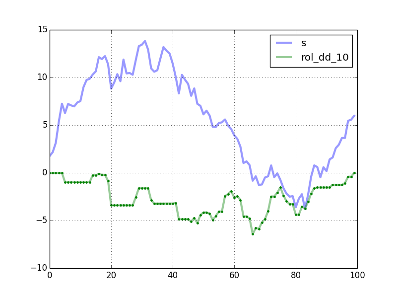
This method also simply encapsulates a function to convert a one-dimensional array into a rolling window view, which can be used elsewhere.
Finding Adaptive Parameters
Many trading strategies based on technical indicators often specify fixed thresholds. For example, some people short when RSI is above 80 and go long when RSI is below 20. Even when applied to indices and industry sectors, such indicators are still not precise enough because, in an upward channel, the RSI peaks will be higher than the RSI peaks in a downward channel; in a downward channel, the RSI bottoms will be much lower than the RSI bottoms in an upward channel.
Furthermore, the RSI value ranges differ for different assets. Not just RSI, many technical indicators require adaptive parameters based on the current market environment and asset.
One solution is to use a Bollinger Bands-like approach, using the upper and lower bounds of the standard deviation of the indicator’s mean. However, this approach implicitly assumes that the data distribution of the technical indicator’s mean follows a normal distribution.
We can relax this condition and instead use quantiles, i.e., Numpy’s percentile, to determine parameter thresholds.
%precision 2
from IPython.core.interactiveshell import InteractiveShell
InteractiveShell.ast_node_interactivity = "all"
np.random.seed(78)
s = np.random.randn(100)
hbound = np.percentile(s, 95)
lbound = np.percentile(s, 5)s[s> hbound]
s[s< lbound]The data exceeding the upper and lower bounds found via percentile is output as follows:
array([2.09, 2.27, 2.21, 2.12, 2.19])
array([-1.68, -2.4 , -1.97, -1.7 , -1.46])Once the indicator exceeds the 95% quantile (hbound), we short; once the indicator falls below the 5% quantile (lbound), we go long.
Here, we can also use the median-based outlier clipping method. Once the indicator exceeds 3 times the median MAD value, a trading signal is issued.