
Pandas for Quant: Alphalens Data Prep & TDX Rolling Functions
“Alphalens requires factor data to be a double-indexed Series and price data to be a DataFrame with dates as the index and asset codes as columns. Using Pandas’ pivot_table and set_index, you can easily perform format conversions to lay the foundation for factor analysis.”
1. Implementing TongDaXin Routines via Rolling Methods
TongDaXin (TDX) is a financial investment software developed by Shenzhen Fortune Trend Technology Co., Ltd., primarily used for market analysis, technical research, and trade execution in stock and futures markets. TDX holds over 80% market share among Chinese brokerages, serving top institutions such as China Merchants Securities and GF Securities. It supports over 50 million investors, with peak concurrent users reaching 8 million, known for its concise interface and rapid market data updates. It is suitable for individual investors, professional traders, and quantitative analysis, particularly in scenarios requiring rapid response to market movements and technical analysis.
rolling is the core method in the Pandas library for executing rolling window calculations, applicable to sliding statistical analysis of time series or DataFrames. Key points include:
- Functionality: Slides over data with a fixed window size (e.g., time periods or number of observations) and performs aggregation or custom calculations (e.g., mean, extrema) within each window.
- Typical Applications: Moving averages, volatility calculation (standard deviation), and technical indicators (e.g., MACD).
Core parameters:
| Parameter | Description |
|---|---|
| window | Window size (integer or time offset, e.g., '5D') |
| min_periods | Minimum number of valid observations in the window; otherwise, returns NaN (defaults to window) |
| center | Window alignment (False for right-aligned, True for centered) |
| win_type | Window weight type (e.g., 'gaussian') |
1.1. HHV (Highest Value in N Periods)
TongDaXin Definition: HHV(X, N) represents the highest value of sequence X over the most recent N periods. This can be implemented in Pandas as follows:
def HHV(s: pd.Series, n: int) -> pd.Series:
return s.rolling(n).max()1.2. LLV (Lowest Value in N Periods)
TongDaXin Definition: LLV(X, N) represents the lowest value of sequence X over the most recent N periods.
def LLV(s: pd.Series, n: int) -> pd.Series:
return s.rolling(n).min()1.3. HHVBARS (Distance from Highest Value to Current Period)
TongDaXin Definition: HHVBARS(X, N) represents the distance (in periods) from the highest value location within the most recent N periods to the current period.
def HHVBARS(s: pd.Series, n: int) -> pd.Series:
def _find_idx(x):
return len(x) - np.argmax(x[::-1]) - 1 if not np.isnan(x).all() else np.nan
return s.rolling(n).apply(_find_idx, raw=True)1.4. LAST (Number of Consecutive Periods Satisfying Condition)
TongDaXin Definition: LAST(X, A, B) indicates that in the past B periods, at least A periods satisfied condition X.
def LAST(condition: pd.Series, a: int, b: int) -> pd.Series:
return condition.rolling(b).sum() >= a1.5. Example
import pandas as pd
import numpy as np
# 导入数据
start = datetime.date(2023, 1, 1)
end = datetime.date(2023, 12, 31)
df = load_bars(start, end)
df.tail()
# 应用函数
df['HHV_5'] = HHV(df['high'], 5) # 5日最高价
df['LLV_5'] = LLV(df['low'], 5) # 5日最低价
df['HHVBARS_5'] = HHVBARS(df['high'], 5) # 最高价距离当前的天数
df['LAST_UP_3_5'] = LAST(df['close'] > df['close'].shift(1), 3, 5) # 5日内至少3日上涨
print(df)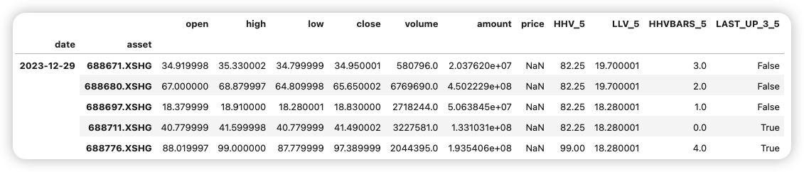
2. Filling Missing Adjustment Factors for Minute-Level Data
In quantitative analysis, when processing minute-level stock data, adjustment factor (forward-adjustment factor) data may be missing. You need to perform nearest-neighbor matching based on time to ensure every minute-level data point has the correct adjustment factor. Adjustment factors are typically adjusted when stocks undergo splits or dividends; these event timestamps may not align exactly with every minute-level timestamp, for example:
- Adjustment factor effective time: 2025-03-27 10:30:00 (event trigger moment)
- Minute-level timestamps: 2025-03-27 10:30:01, 10:30:02 (trading data)
Tip
Traditional `merge` or `join` methods cannot match such temporally adjacent but non-strictly equal data. You must use the **as-of join** feature. `merge_asof` finds the most recent adjustment factor prior to each minute-level timestamp, ensuring correct application of adjustments.2.1. Basic Syntax and Examples
2.1.1. Basic Syntax
pd.merge_asof(
left, # 左表(分钟线数据)
right, # 右表(复权因子数据)
on='time', # 时间列名(必须排序)
direction='backward', # 匹配方向:向前/向后/最近
tolerance=pd.Timedelta('1min'), # 最大时间差
allow_exact_matches=True # 是否允许精确匹配
)2.1.2. Basic Example
import pandas as pd
import numpy as np
# 生成示例数据(假设复权因子在非整分钟时间点更新)
minute_data = {
'time': [
'2025-03-27 10:29:58', # 完整日期+时间
'2025-03-27 10:30:01',
'2025-03-27 10:30:03',
'2025-03-27 10:30:05',
'2025-03-27 10:30:08' # 确保所有时间包含日期
],
'price': [100.2, 101.5, 102.0, 101.8, 103.2]
}
df_trade = pd.DataFrame(minute_data).sort_values('time')
adjust_data = {
'time': [
'2025-03-27 10:29:55',
'2025-03-27 10:30:00',
'2025-03-27 10:30:06'
], 'adjust_factor': [1.0, 0.95, 1.02]
}
df_adjust = pd.DataFrame(adjust_data).sort_values('time')
# 强制转换为 datetime 类型(处理混合格式)
df_trade['time'] = pd.to_datetime(
df_trade['time'],
format='%Y-%m-%d %H:%M:%S',
errors='coerce'
)
df_adjust['time'] = pd.to_datetime(
df_adjust['time'],
format='%Y-%m-%d %H:%M:%S',
errors='coerce'
)
assert df_trade['time'].dtype == 'datetime64[ns]', "交易数据时间列转换失败"
assert df_adjust['time'].dtype == 'datetime64[ns]', "复权因子时间列转换失败"
# 关键步骤:按时间向前匹配最近的复权因子
merged = pd.merge_asof(
df_trade,
df_adjust,
on='time',
direction='backward', # 取<=当前时间的最近值
tolerance=pd.Timedelta(minutes=1) # 最多允许1分钟间隔
)
merged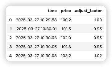
2.2. Advanced Techniques
2.2.1. Multi-Asset Matching (Grouping by Stock Code)
# 假设数据包含多只股票
merged = pd.merge_asof(
df_trade.sort_values('time'),
df_adjust.sort_values('time'),
on='time',
by='symbol', # 按股票代码分组匹配
direction='backward'
)2.2.2. Dynamically Adjusting Factor Effective Time
If the adjustment factor’s effective time needs to be advanced or delayed, preprocess the right table’s time:
df_adjust['time'] = df_adjust['time'] + pd.Timedelta(seconds=30) # 延后30秒生效
df_adjust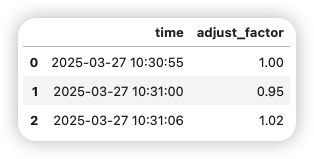
2.2.3. Handling Missing Values
merged['adjust_factor'] = merged['adjust_factor'].ffill() # 前向填充缺失值2.3. Comparison with Other Methods
| Method | Applicable Scenario | Advantages | Disadvantages |
|---|---|---|---|
| merge_asof | Temporally adjacent match | High efficiency for non-aligned timestamps | Requires pre-sorted data |
| merge | Exact time match | Precise results | Cannot handle time deviations |
| concat | Simple stacking | Fast merging | Does not handle time relations |
3. Preparing Data for Alphalens
When using Alphalens for factor analysis, we often need to organize factor and price data into specific formats. Alphalens requires factor data to be a Series with a double index (date and asset), while price data must be a DataFrame with dates as rows, asset codes as columns, and prices as values. This is critical; incorrect formats will cause Alphalens to throw errors.
Therefore, we need to know how to convert raw data into this format. Here, we consider using pivot_table to transform price data and set_index to create the double index for factor data.
3.1. Data Format Specifications (Alphalens Mandatory Requirements)
3.1.1. Factor Data Format
You must construct a double-indexed Series, with index order: Date -> Asset Code, and values as factor values:
# 原始数据示例(含日期、股票代码、因子值)
raw_factor = pd.DataFrame({
'date': ['2025-03-25', '2025-03-25', '2025-03-26', '2025-03-26'],
'symbol': ['AAPL', 'MSFT', 'AAPL', 'MSFT'],
'value': [0.5, -0.3, 0.7, 0.2]
})
# 转换为Alphalens格式
factor = raw_factor.set_index(['date', 'symbol'])['value']
factor.index = pd.MultiIndex.from_arrays(
# 确保日期为datetime类型
[pd.to_datetime(factor.index.get_level_values('date')),
factor.index.get_level_values('symbol')]
)
factor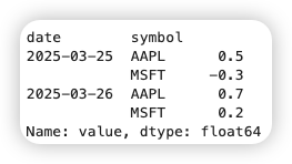
3.1.2. Price Data Format
You must construct a DataFrame with dates as the index and asset codes as column names:
# 原始数据示例(含日期、股票代码、收盘价)
raw_price = pd.DataFrame({
'date': ['2025-03-25', '2025-03-25', '2025-03-26', '2025-03-26'],
'symbol': ['AAPL', 'MSFT', 'AAPL', 'MSFT'],
'close': [150, 280, 152, 285]
})
# 转换为Alphalens格式
prices = raw_price.pivot(index='date', columns='symbol', values='close')
prices.index = pd.to_datetime(prices.index) # 日期转换为datetime类型
3.2. Key Preprocessing Operations
3.2.1. Time Index Alignment
# 检查时间范围是否重叠
print("因子时间范围:",factor.index.get_level_values('date').min()
, "~", factor.index.get_level_values('date').max())
print("价格时间范围:",prices.index.min(), "~", prices.index.max())# 若存在时间缺口,用前向填充(避免未来数据)
prices = prices.ffill()3.2.2. Outlier Handling
# Winsorize去极值(保留98%数据)
factor_clipped = factor.clip(
lower=factor.quantile(0.01),
upper=factor.quantile(0.99)
)
# 标准化处理(Z-score)
factor_normalized = (factor - factor.mean()) / factor.std()3.2.3. Missing Value Handling
# 删除缺失值超过50%的资产
valid_symbols = factor.unstack().isnull().mean() < 0.5
factor = factor.loc[:, valid_symbols[valid_symbols].index.tolist()]
# 前向填充剩余缺失值
factor = factor.groupby(level='symbol').ffill()3.3. Advanced Operation Techniques
3.3.1. Multi-Factor Processing
# 假设存在动量因子和市值因子
factor_mom = ... # 动量因子数据
factor_size = ... # 市值因子数据
# 横向拼接为MultiIndex列
combined = pd.concat(
[factor_mom.rename('momentum'), factor_size.rename('size')],
axis=1
)
# 转换为双层索引
combined = combined.stack().swaplevel(0, 1).sort_index()3.3.2. Sector Neutralization
# 假设有行业分类数据
industries = pd.Series({
'AAPL': 'Technology',
'MSFT': 'Technology',
'XOM': 'Energy'
}, name='industry')
# 按行业分组标准化
factor_neutral = factor.groupby(
industries, group_keys=False
).apply(lambda x: (x - x.mean()) / x.std())3.4. Data Validation and Interface Integration
3.4.1. Format Validation
# 检查因子索引层级
assert factor.index.names == ['date', 'symbol'], "因子索引命名错误"
# 检查价格数据类型
assert prices.columns.dtype == 'object', "价格数据列名应为资产代码"3.4.2. Alphalens Interface Calls
from alphalens.utils import get_clean_factor_and_forward_returns
# 生成分析数据集
factor_data = get_clean_factor_and_forward_returns(
factor=factor,
prices=prices,
periods=(1, 5, 10), # 1/5/10日收益率
quantiles=5, # 分为5组
filter_zscore=3 # 剔除3倍标准差外的异常值
)
# 生成完整分析报告
import alphalens
alphalens.tears.create_full_tear_sheet(factor_data)3.5. Common Issue Solutions
| Issue Description | Solution |
|---|---|
| ValueError: Price data contains future info | Check if price timestamps are later than factor timestamps; shift prices by one period using prices = prices.shift(1) |
| KeyError: Asset code mismatch | Use prices.columns.intersection(factor.index.get_level_values('symbol')) to take the intersection |
| Blank charts | Run in Jupyter Notebook and add the %matplotlib inline magic command |
Through the above operations, you can efficiently convert raw data to Alphalens-compatible formats, ensuring the accuracy of factor analysis. In practical applications, it is recommended to test on small sample data first before expanding to full datasets.