Scaling and Normalization in Quant Strategies: Beyond ML

中文 📅 2023-12-13 👁 views this month —

Scaling and normalization are inevitable challenges in machine learning. In quantitative trading, we frequently encounter similar issues, regardless of whether machine learning is employed.

This article serves as a summary of Lesson 12 from the Da Mao Weng Quantitative Finance Practical Course, incorporating new insights to form a standalone piece.

Mathematically, scaling (or normalization) is the process of mapping values from one range to another. This mapping can be linear (e.g., min-max scaling) or non-linear. For instance, we often need to map an interval of $(-\infin, +\infin)$ to $(-1, 1)$ or $(0, 1)$.

From a quantitative trading perspective, the Williams %R (WR) indicator is a classic example of min-max scaling, defined as:

$$ WR = \frac{max(high) - close}{max(high) - min(low)} $$

attention

Extreme caution is required when using min-max scaling in quantitative trading.
It presents two primary issues.
First, it may introduce look-ahead bias (future data), although this isn't always the case. For example, Williams %R calculated in real-time does not use future data; however, in backtesting, whether it introduces look-ahead bias depends on the implementation.
Second, predictions based on min-max scaled data are constrained to the $[min, max]$ interval. However, stock prices do not have fixed minimums or maximums. If we predict future prices based on current scaled data, the predicted price cannot exceed the current observed maximum, whereas in reality, stock prices can rise indefinitely.
In contrast, when applying min-max scaling to the Iris dataset's petal length and width, the sampling generally represents the population well, making it unlikely for future data to significantly exceed the sampled min/max.

More often, quantitative analysis requires non-linear mapping. For example, we have previously discussed that extremely low volume ("ground volume") is a significant trading signal: "Low volume signals low prices." What constitutes "ground volume"? We can measure it by the number of periods since the lowest volume. This value has a minimum of 1 and a maximum that could be 10 days, a month, a year, or longer. Mathematically, its range is $[1, +\infin)$.

In Lesson 13, when discussing the evaluation function for the "rounded bottom" pattern, we noted that the width interval might range from $[3, +\infin)$.

For such uncertain value ranges, we typically use S-shaped functions for transformation. These include:

$$ f(x) = sigmoid(x) = \frac{1}{1 + e^{-x}} \tag 1 $$

$$ f(x) = tanh(x) = \frac{e^x - e^{-x}}{e^x + e^{-x}} \tag 2 $$

$$ f(x) = \frac{x}{1+|x|} \tag 3 $$

$$ f(x) = \frac{x}{sqrt(1 + x^2)} \tag 4 $$

In special cases where sampled data exhibits periodic characteristics, and we wish to preserve periodic correlations after transformation, we can use $sin$ and $cos$ functions. This normalization method was employed in the seminal paper Attention Is All You Need (for encoding token positions):

Considering the periodic nature of stock price fluctuations, similar methods might find application in quantitative trading.

However, using sigmoid functions for normalization has drawbacks. Take the "ground volume" example: the signal meaning of ground volume over 13 periods differs significantly from that over 120 periods. A stock easily experiences ground volume within 13 periods, but rarely within 120 periods. When it does occur, it often triggers a rebound of a certain magnitude.

If we apply sigmoid normalization, their normalized values would be identical:

1234def sigmoid(x):
    return 1/(1 + np.exp(-x))

print("sigmoid(12) == sigmoid(13)?", np.isclose(sigmoid(12), sigmoid(13)))

As shown above, when $x > 12$, we can no longer distinguish differences in function values during computation.

Therefore, in practice, we often modify the sigmoid function to maintain high response sensitivity within a specific interval. The formula is:

$$ f(x) = \frac{2}{1+e^{-\frac{ln(40000)}{b}.(x-b)+ln(0.005)}} - 1 $$

The shape of the graph is primarily determined by parameter $b$. When $b=15$, the graph is as follows:

50%

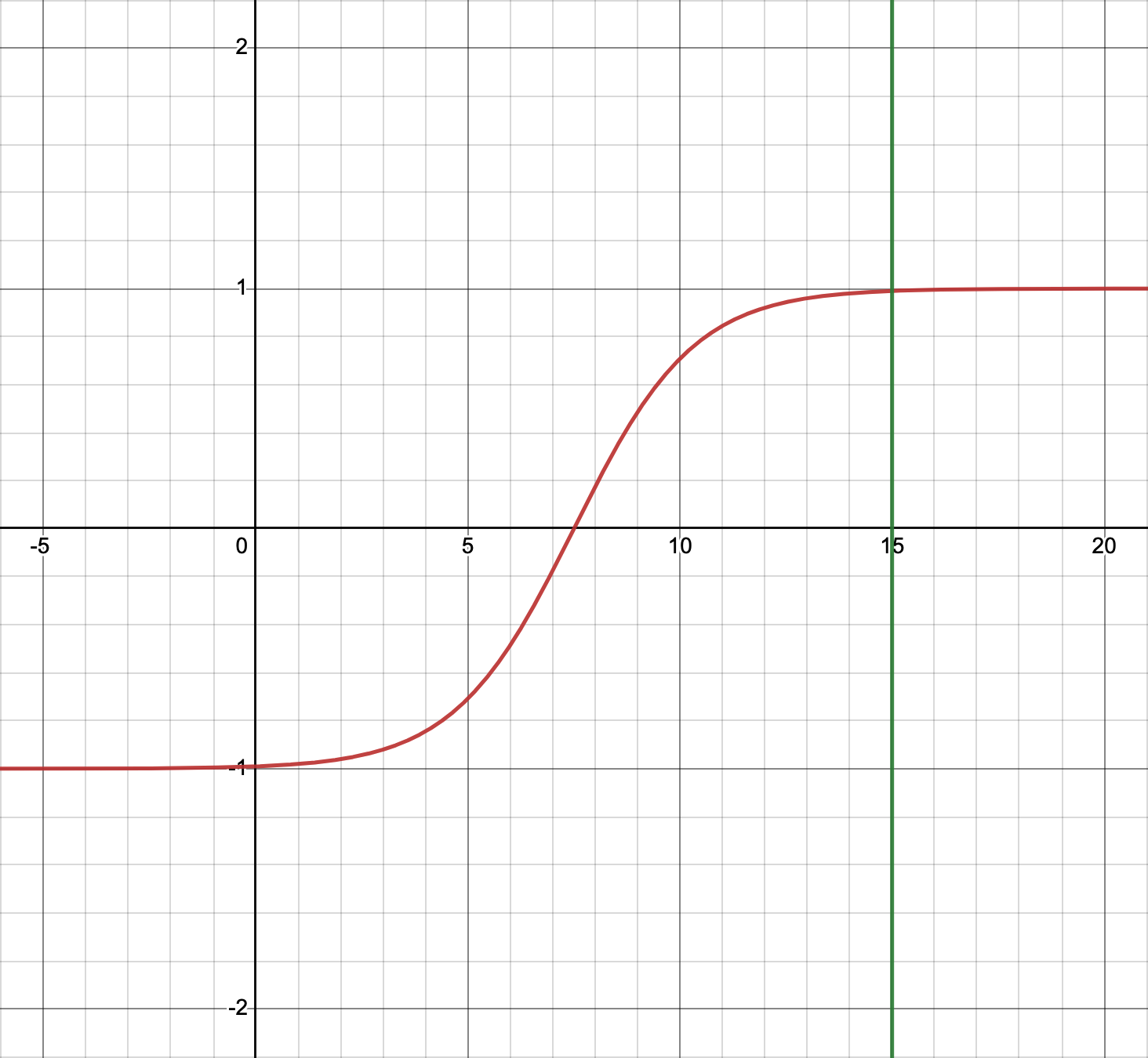
The distribution range is $[-1, 1]$, with high distribution density when $x$ is in $[0, b]$.

In non-machine-learning quantitative scoring strategies, we may prefer function values to fall within $[0, 1]$ (consider that both RSI and WR operate in this range, not $[-1, 1]$). Thus, we slightly modify the above formula, with the code implementation as follows:

12345678910111213141516171819202122232425262728import matplotlib.pyplot as plt

def scaled_sigmoid(x, start, end):
    """当`x`落在`[start,end]`区间时，函数值为[0,1]且在该区间有较好的响应灵敏度
    """
    n = np.abs(start - end)

    score = 2/(1 + np.exp(-np.log(40_000)*(x - start - n)/n + np.log(5e-3)))
    return score/2


fig, (ax1, ax2, ax3,ax4) = plt.subplots(nrows = 1, ncols = 4, figsize=(12,3))

x = np.linspace(0, 1)
ax1.plot(x, [scaled_sigmoid(i, x[0], x[-1]) for i in x])
ax1.set_title("fit (0,1)")

x = np.linspace(0, 100)
ax2.plot(x, [scaled_sigmoid(i, x[0], x[-1]) for i in x])
ax2.set_title("fit (0, 100)")

x = np.linspace(18, 38)
ax3.plot(x, [scaled_sigmoid(i, x[0], x[-1]) for i in x])
ax3.set_title("fit (18, 38)")

x = np.linspace(0, 100)
ax4.plot(x, [sigmoid(i) for i in x])
ax4.set_title("fit (0,100) with original")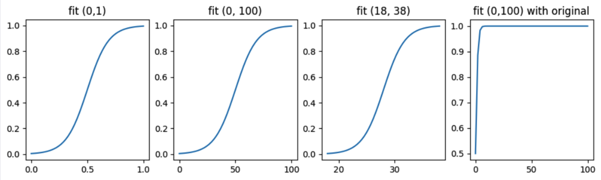

As seen in the graph above, compared to the original sigmoid, the new scaled_sigmoid function exhibits excellent response sensitivity within the $[start, end]$ interval, where the distribution density is highest.