Tushare vs East Money: The Hidden Bias in Daily Returns

I’m currently building a quantitative framework for personal use, sourcing data from Tushare and using QMT for real-time market data and trading APIs. While testing a strategy, I noticed that signals weren’t triggering when they should have. This led to a debugging journey that uncovered a startling issue: even the most basic daily return data was inconsistent.

What Should Yesterday’s Return Have Been?

import akshare as ak import tushare as ts import pandas as pd import matplotlib.pyplot as plt import time

start = "20240101" end = "20241231"

symbol_ak = "000001" symbol_ts = "000001.SZ"

pro = ts.pro_api()

A robust quantitative framework must support local data storage. For market data, we typically store unadjusted prices and adjustment factors, calculating the required adjusted prices on the fly.

In Tushare, we obtain daily unadjusted prices and daily returns via the pro.daily interface:

12345df_ts = pro.daily(ts_code = symbol_ts, start_date = start, end_date = end)
df_ts.index=pd.to_datetime(df_ts["trade_date"])

df_ts.sort_index(inplace=True)
df_ts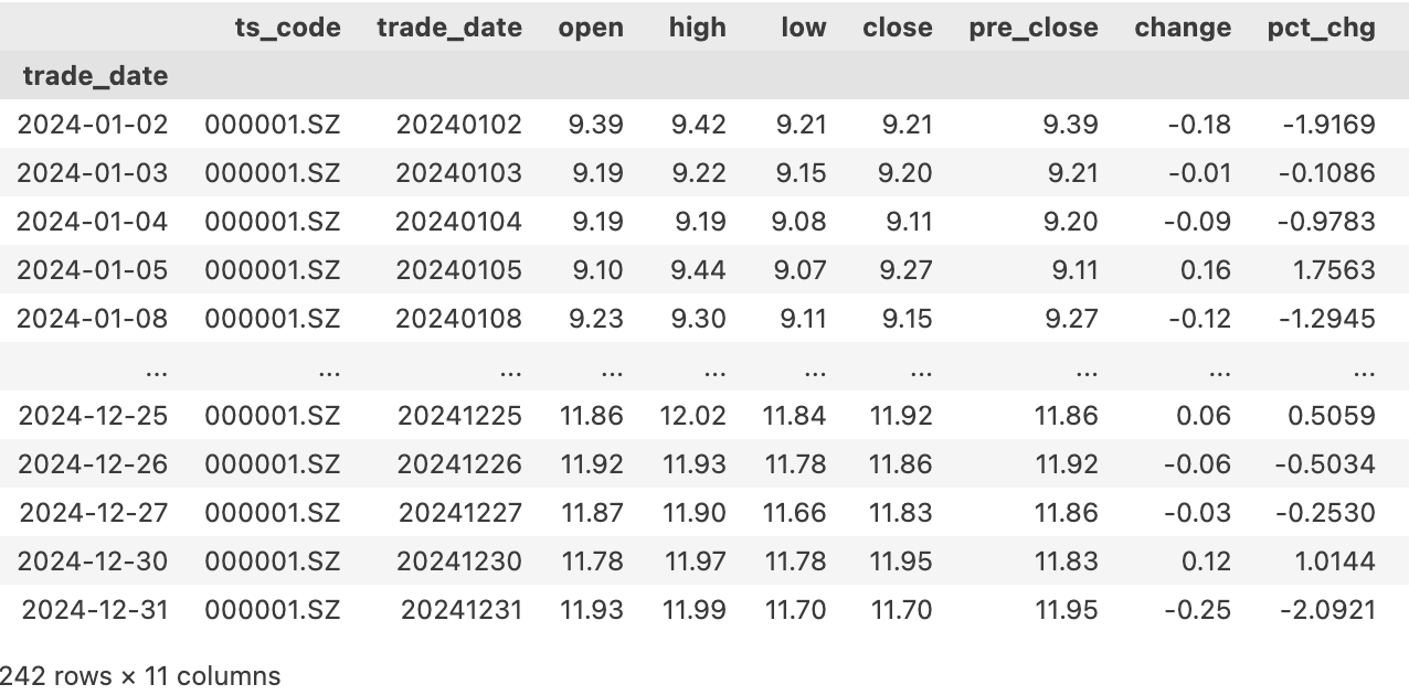

However, when I compared these returns with those from East Money (Dongfang Caifu), I found a discrepancy:

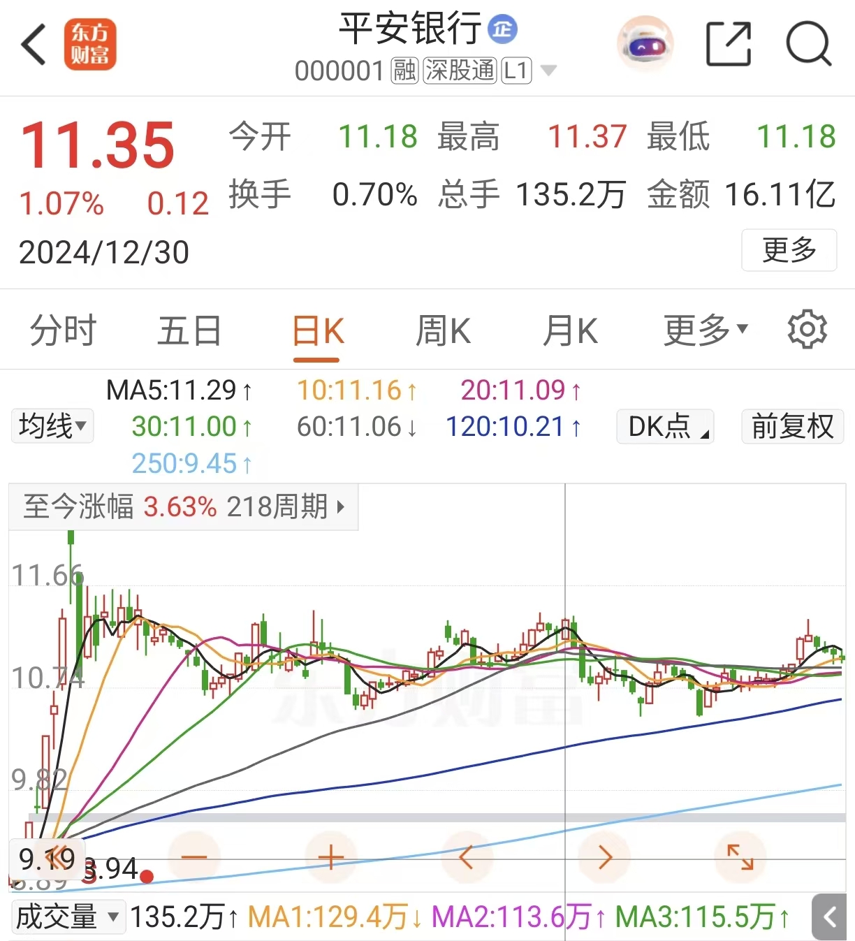
On December 31, East Money reported that Ping An Bank rose by 1.07%, while Tushare indicated a rise of 1.01%. This wasn’t the largest discrepancy. The biggest gap occurred on February 11, where Tushare reported a 9.97% gain, while East Money reported an 11.86% gain—a difference of nearly 2 percentage points.

For a single stock, can one day show a 1% gain and another day show a 2% gain, both from authoritative software? Isn’t this surreal?

How Are Returns Calculated?

Theoretically, the daily return is calculated as $(Close_{T+1} / Close_T) - 1$. Considering corporate actions, we must first adjust the closing prices before calculating returns. In practice, adjustment only affects the return on the ex-dividend/ex-rights date itself. Therefore, when no corporate action occurs, the return calculated using unadjusted prices is identical to that calculated using adjusted prices.

Let’s verify this. We need the adj_factor interface to obtain individual stock adjustment factors.

1234567891011121314adjust_ts = pro.adj_factor(ts_code=symbol_ts, trade_date='')
adjust_ts.index = pd.to_datetime(adjust_ts["trade_date"])
adjust_ts.sort_index(inplace=True)

# Merge into main dataframe
df_ts["adjust"] =  adjust_ts.query("index >= '2024-01-01' and index <= '2024-12-31'")["adj_factor"]

# Calculate daily returns
adjust_close = df_ts["close"] * df_ts["adjust"]/df_ts["adjust"][-1]
df_ts["pct_chg_v2"] = adjust_close.pct_change().round(4)*100

# Display key columns
cols = ["close", "pre_close", "adjust", "pct_chg", "pct_chg_v2"] 
df_ts[cols]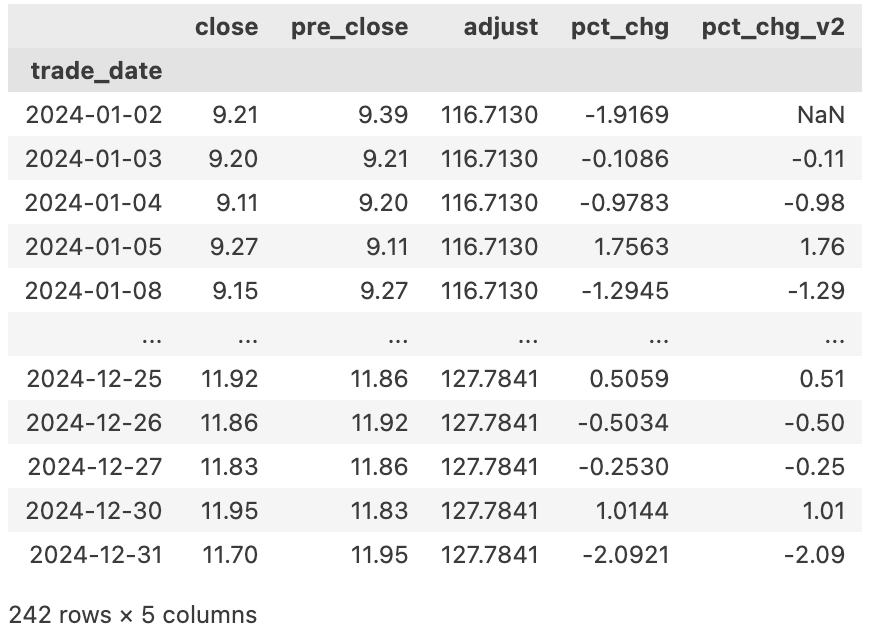

As shown, the daily returns in Tushare’s daily interface are indeed calculated using adjusted closing prices. We can visualize the difference between the two sequences using the following code:

123456789101112131415161718192021222324252627282930def compare(df1, col1, col2, df2=None, title=""):
    if df2 is not None:
        df = pd.DataFrame({
            col1: df1[col1],
            col2: df2[col2]
        }, index=df1.index)

    else:
        df = df1[[col1, col2]]

    fig, (ax1, ax2) = plt.subplots(1, 2, figsize=(14, 6), sharey=True)

    ax1.scatter(df[col1].round(2), df[col2].round(2), alpha=0.6, s=30, color="#1f77b4")

    x_min = min(df[col1].min(), df[col2].min())
    x_max = max(df[col1].max(), df[col2].max())
    ax1.plot([x_min, x_max], [x_min, x_max], "r--", lw=2, label="y = x")

    df.plot(ax=ax2)

    ax1.set_xlabel(col1, fontsize=12)
    ax1.set_ylabel(col2, fontsize=12)

    fig.suptitle(title, fontsize=14)
    plt.legend()
    plt.grid(alpha=0.3)
    plt.axis("equal")  # Equal x/y axis scaling to avoid visual distortion
    plt.show()

compare(df_ts, "pct_chg", "pct_chg_v2", title="Comparison of Original vs Adjusted Closing Price Returns")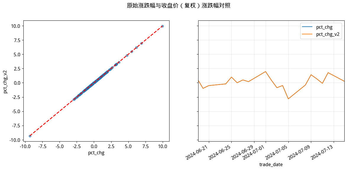

Clearly, the two sequences are identical. This confirms that we don’t need to rely on the daily interface’s returned daily returns; instead, we can calculate daily returns solely using saved unadjusted closing prices and adjustment factors. This aligns with most tutorials and quantitative frameworks.

Since the calculation method is correct, is the discrepancy between Tushare’s returns and East Money’s data merely an isolated error?

Bringing AkShare to Testify

Comparing data bar-by-bar via market software is inefficient. We need a more robust method to acquire market data. For East Money’s data, the most reliable approach is through AkShare.

In AkShare, we retrieve market data via stock_zh_a_hist. This interface returns daily returns via the "涨跌幅" (daily change %) field. While carefully reading AkShare’s documentation, I unexpectedly discovered that the example provided in the official documentation shows different daily returns under three different adjustment modes!

Below, we will use three adjustment modes to obtain all return data, allowing you to intuitively feel the differences.

The following content requires AkShare. Due to web scraping mechanisms, it may run unstably on the Kuangti Research Platform.

1234567891011121314151617181920212223data = []

# Unadjusted
df_ak_no_fq = ak.stock_zh_a_hist(symbol=symbol_ak, start_date=start,end_date=end, adjust="")
df_ak_no_fq.index = pd.to_datetime(df_ak_no_fq["日期"])
time.sleep(0.2)

data.append(df_ak_no_fq["涨跌幅"].rename("ak_no_fq"))

# Forward-adjusted (Pre-adjusted)
df_ = ak.stock_zh_a_hist(symbol=symbol_ak, start_date=start,end_date=end, adjust="qfq")
df_.index = pd.to_datetime(df_["日期"])
data.append(df_["涨跌幅"].rename("ak_qfq"))
time.sleep(0.2)

# Backward-adjusted (Post-adjusted)
df_ = ak.stock_zh_a_hist(symbol=symbol_ak, start_date=start,end_date=end, adjust="hfq")
df_.index = pd.to_datetime(df_["日期"])
data.append(df_["涨跌幅"].rename("ak_hfq"))

df_ak = pd.concat(data, axis=1)
df_ak.index = df_ak_no_fq.index
df_ak

This gives us the various return series under AkShare.

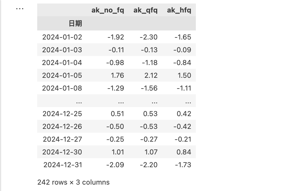
Since AkShare’s data is scraped from East Money’s web pages (including APIs), the data we obtain is essentially the same as that from the East Money market software. Among these data series, the returns under the forward-adjusted (pre-adjusted) column match what we see in the East Money software. Therefore, let’s compare this column with the Tushare returns we obtained earlier:

compare(df_ak, "ak_qfq", "pct_chg", df_ts, title="Ak Forward-Adjusted vs Tushare")

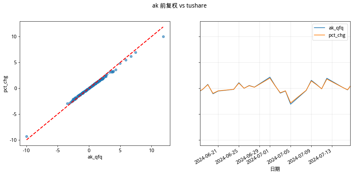
As shown, the two return series are largely inconsistent. The question is: Is East Money correct, or is Tushare?

The answer lies in the return data obtained from AkShare. We know that for the same instrument on the same day, a stock cannot have multiple daily returns; applying adjustments to daily returns is meaningless. After various adjustments, the calculated returns on dates without corporate actions should be identical to the unadjusted returns.

Now, let’s compare the unadjusted returns from AkShare with the returns from Tushare.

compare(df_ak, "ak_no_fq", "pct_chg", df_ts, title="AkShare Unadjusted vs Tushare")

From the left chart, we can see that only two points differ.

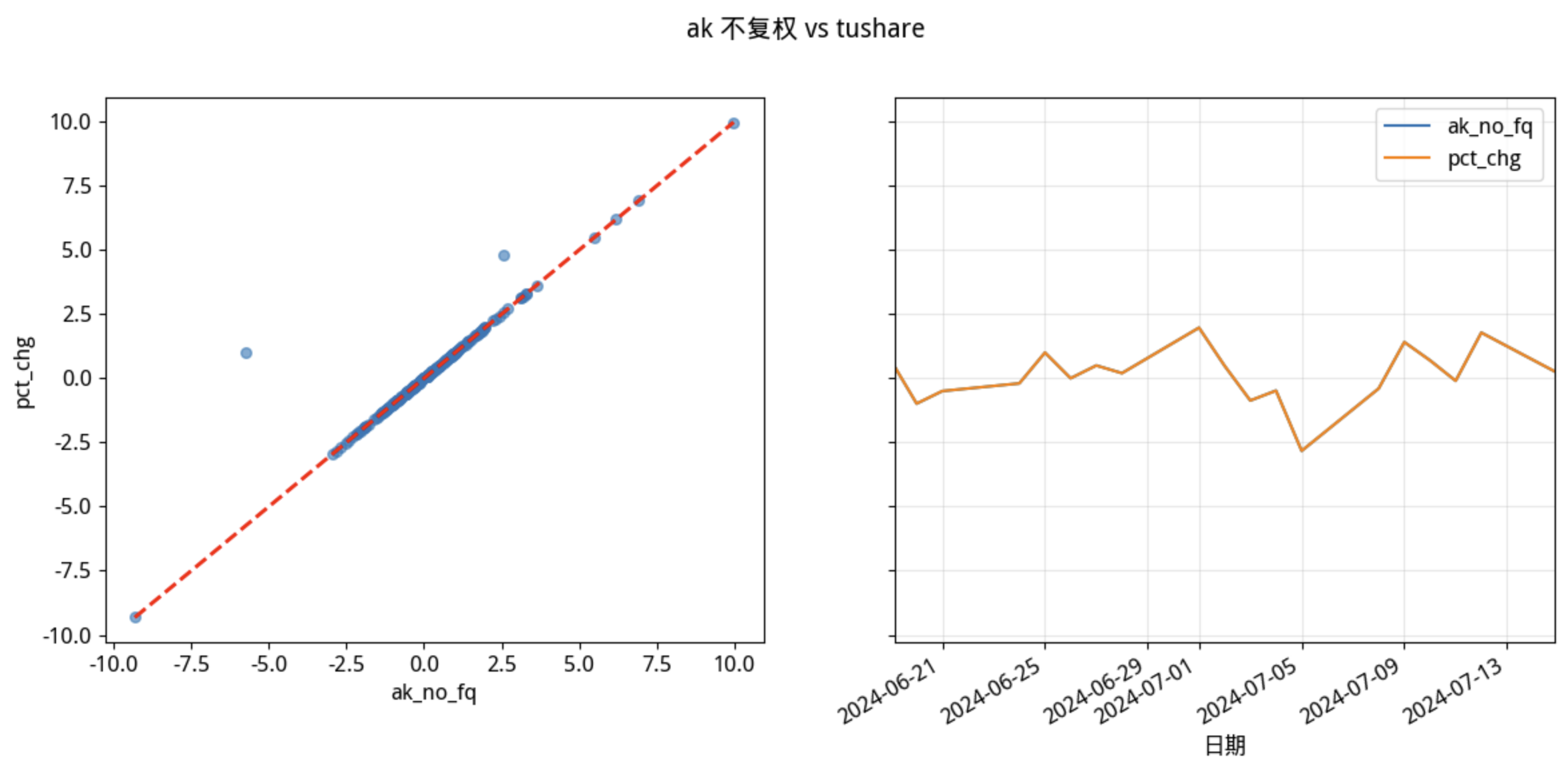
The Final Proof

Tushare’s daily interface also returns pre_close (previous close) data.

12345from pandas.testing import assert_series_equal

by_pre_close = ((df_ts["close"]/df_ts["pre_close"] - 1)*100).round(2)

assert_series_equal(by_pre_close, df_ts["pct_chg"], atol=1e-2, check_names = False)

The returns calculated from $Close / PreClose$ are identical to the daily returns returned by the interface. Since its unadjusted close and pre_close are both correct, Tushare’s data is accurate. East Money’s data (or the data obtained via AkShare) deviates from our expectations. Its unadjusted daily returns are truly unadjusted: if a stock’s actual receipt was 5 yuan yesterday, and it opens 10% higher today, but a 1:1 rights issue occurs, resulting in an actual receipt price of 2.75 yuan, East Money would calculate the daily return as -45%.

However, its forward-adjusted (pre-adjusted) daily returns—which is the default view in market software—undergo some form of processing (I’m unsure if it’s true adjustment). Therefore, at the moment I wrote this article, Ping An Bank’s actual gain on February 11, 2024, was 9.97%, but it would display as an 11.86% gain in the East Money software. East Money’s handling of this has its reasons, but from a quant’s perspective, it may not align with our expectations.

There’s a saying: "He who controls the past controls the future; he who controls the present controls the past." In East Money’s default view, this seems to hold true. However, quants believe that a stock’s daily return should be a fixed, immutable value. It should not change over time; it is not Schrödinger’s cat, where observing it at different times yields different results.

We have already obtained Tushare’s adjustment data. We can visually identify the dates of corporate actions using the following chart:

1df_ts.adjust.plot()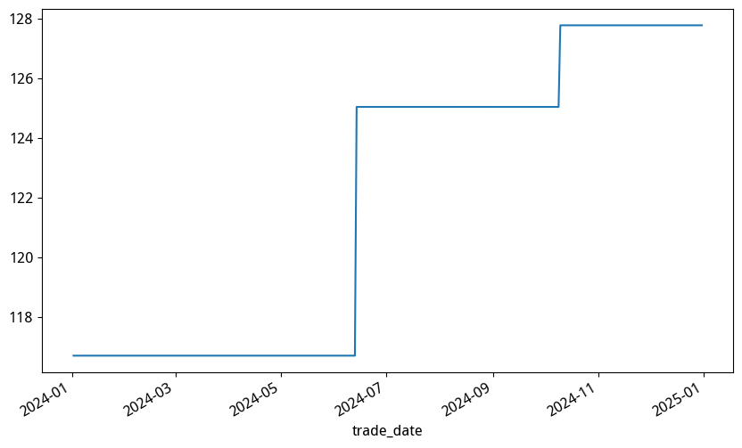

In the 'AkShare Unadjusted vs Tushare' chart, the two points deviating from the baseline correspond exactly to these two jumps.

Quantitative trading is a precise discipline that demands meticulous scrutiny of every detail. Through today’s discussion, you’ve learned that while East Money’s data is generally accurate, using its returned daily returns (whether unadjusted or adjusted) as training targets can introduce significant systematic bias.

On this path, you need Kuangti and...

Conclusion

Quantitative trading is a precise discipline that demands meticulous scrutiny of every detail. Through today’s discussion, you’ve learned how data discrepancies can introduce systematic bias and understood how to verify data reliability using adjustment factors and data comparisons.

If you’re passionate about quantitative trading and want to delve deeper into factor mining, strategy construction, and model optimization, consider joining our Quantitative 24 Lessons. This course is designed specifically for quantitative enthusiasts, guiding you from basics to advanced topics to master the core skills of quantitative trading. Let’s explore the world of quantitative finance together and discover more possibilities!