
Low Volume, Low Price? Backtesting Shanghai Index Data

The stock market adage goes: "High volume signals high price; low volume signals low price." Today, let’s put this to the test.
To quantify this adage, we must first solve a computational problem: What is the number of periods since the $i$-th element in an array became the minimum (or maximum)?
Consider the following array: 1, 2, 2, 1, 3, 0.
- The 1st element,
1, is the minimum over the last 1 period. - The 2nd element,
2, is the maximum so far, and thus also the minimum over the last 1 period. - The 4th element,
1, is the minimum since the 2nd element, meaning it is the minimum over the last 3 periods.
Calculating this sequentially yields the sequence: 1, 1, 2, 1, 4, 6. Each item represents the number of periods since the corresponding element in the original array was the minimum up to that point.
What is the use of this algorithm? It can be applied in the following calculations.
For instance, consider the adage: "High volume signals high price; low volume signals low price."
When prices are high, a surge in trading volume (high volume) over a period may be unsustainable, often leading to a decline. Conversely, when prices are low, a drop in trading volume (low volume) indicates extreme market apathy. At this stage, prices are susceptible to manipulation, attracting speculative capital. To calculate "low volume," we need to know how many periods the current trading volume has been the minimum.
For example, if the market's current trading volume becomes the lowest in 120 days, it is likely to attract attention. To verify whether a rally follows such "low volume" conditions, we need to perform factor analysis or backtest the strategy. The question now is: how do we calculate this efficiently?
The Naive Double Loop
Using the array above, the simplest algorithm uses nested loops:
def min_range_loop(s):
minranges = [1]
for i in range(1, len(s)):
for j in range(i-1, -1, -1):
if s[j] < s[i]:
minranges.append(i - j)
break
else:
minranges.append(i+1)
return minranges
s = [1,2,2,1,3,0]
min_range_loop(s)The output is: 1, 1, 2, 1, 4, 5.
This implementation uses a double loop and is likely time-consuming. When we generate an array with 10,000 elements and run it, we find that a single call takes 9.5ms.
Insights from myTT
The myTT library contains a similar function implementation:
def LOWRANGE(S):
# LOWRANGE(LOW) indicates how many periods the current lowest price has been the minimum by jqz1226
rt = np.zeros(len(S))
for i in range(1,len(S)): rt[i] = np.argmin(np.flipud(S[:i]>S[i]))
return rt.astype('int')This function also implements finding how many periods ago the $i$-th element was the minimum, though the comments suggest it is primarily used for calculating the lowest price. In reality, the sequence s does not matter.
This function uses a single loop and the flipud function, which is quite clever. The usage demonstration is as follows:
s = [1, 2, 2, 3, 2, 0]
np.all(np.flipud(s) == s[::-1])Its actual function is simply to reverse the array.
However, the LOWRANGE function seems to fail to implement its declared functionality. I suspect there might be a misunderstanding of its purpose. When we test it with the same array, the results do not match those from the double-loop approach.
s = np.array([1, 2, 2, 3, 2, 0])
LOWRANGE(s)The result is:
array([0, 0, 0, 0, 1, 0])Furthermore, if we perform a performance test on an array with 10,000 elements, LOWRANGE takes 60ms, losing to the Python double loop. The test environment used Python 3.11, which shows significant optimization improvements.
So, how should we completely eliminate loops?
The Brain-Bending Vectorization
If we can expand the array [1, 2, 2, 3, 2, 0] into:
$\displaystyle \left[\begin{matrix}1.0 & \text{NaN} & \text{NaN} & \text{NaN} & \text{NaN} & \text{NaN}\1.0 & 2.0 & \text{NaN} & \text{NaN} & \text{NaN} & \text{NaN}\1.0 & 2.0 & 2.0 & \text{NaN} & \text{NaN} & \text{NaN}\1.0 & 2.0 & 2.0 & 3.0 & \text{NaN} & \text{NaN}\1.0 & 2.0 & 2.0 & 3.0 & 2.0 & \text{NaN}\1.0 & 2.0 & 2.0 & 3.0 & 2.0 & 0.0\end{matrix}\right]$
and implement a function that accepts this matrix input and independently calculates how many periods the last column of each row represents the minimum, the problem is solved.
To achieve this, we can use numpy's masked arrays and triu matrices.
n = len(s)
mask = np.triu(np.ones((n, n), dtype=bool), k=1)
masked = np.ma.array(m, mask=mask)
maskedThe k parameter in triu determines the position of the main diagonal in the generated triangular matrix. If k=0, the diagonal is on the main diagonal; if k<0, the diagonal is k units below the main diagonal; if k>0, the diagonal is k units above the main diagonal.
We obtain the following output:
masked_array(
data=[[1.0, --, --, --, --, --],
[1.0, 2.0, --, --, --, --],
[1.0, 2.0, 2.0, --, --, --],
[1.0, 2.0, 2.0, 3.0, --, --],
[1.0, 2.0, 2.0, 3.0, 2.0, --],
[1.0, 2.0, 2.0, 3.0, 2.0, 0.0]],
mask=[[False, True, True, True, True, True],
[False, False, True, True, True, True],
[False, False, False, True, True, True],
[False, False, False, False, True, True],
[False, False, False, False, False, True],
[False, False, False, False, False, False]],
fill_value=1e+20)Parts where the mask flag is True will not participate in calculations. If we pass masked to sympy, we can verify this:
from sympy import Matrix
n = len(s)
mask = np.triu(np.ones((n, n), dtype=bool), k=1)
masked = np.ma.array(m, mask=mask)
Matrix(masked)We obtain the expanded matrix as expected.
$\displaystyle \left[\begin{matrix}1.0 & \text{NaN} & \text{NaN} & \text{NaN} & \text{NaN} & \text{NaN}\1.0 & 2.0 & \text{NaN} & \text{NaN} & \text{NaN} & \text{NaN}\1.0 & 2.0 & 2.0 & \text{NaN} & \text{NaN} & \text{NaN}\1.0 & 2.0 & 2.0 & 3.0 & \text{NaN} & \text{NaN}\1.0 & 2.0 & 2.0 & 3.0 & 2.0 & \text{NaN}\1.0 & 2.0 & 2.0 & 3.0 & 2.0 & 0.0\end{matrix}\right]$
Now, the problem we need to solve is: for each row, how many periods does the last number represent the minimum? We perform a transformation:
s = np.array([1, 2, 2, 3, 2, 0])
diff = s[-1] - s
rng = np.arange(len(diff))
rng - np.argmax(np.ma.where(diff > 0, rng, -1))We subtract the last element from the array, then compare if elements are greater than zero. If so, we set the value to the index (rng); otherwise, we set it to -1. Then, we use argmax to find the last non-zero value. The last value of the output element is the minimum period count. In this example, it is 5.
If s = np.array([1, 2, 2, 3, 2]), the calculated last value is 4.
If s = np.array([1, 2, 2, 3]), the calculated last value is 1.
And so on. This exactly matches the result of calculating along axis=1 in the masked array.
Here is the complete code:
def min_range(s):
"""Calculate how many periods prior to element i the minimum value occurred in sequence s"""
n = len(s)
diff = s[:,None] - s
mask = np.triu(np.ones((n, n), dtype=bool), k=1)
masked = np.ma.array(diff, mask=mask)
rng = np.arange(n)
ret = rng - np.argmax(np.ma.where(masked > 0, rng, -1), axis=1)
ret[0] = 1
if filled[1] <= filled[0]:
ret[1] = 2
return retLet's verify the results:
s = np.array([1, 2, 2, 3, 2, 0])
min_range(s)The output is 1, 1, 2, 1, 4, 6.
There is a slight discrepancy in the last number compared to the loop version. However, when looking for "low volume" conditions, this value generally needs to be large to be effective, so a small error is acceptable.
Eliminating two loops should significantly improve performance, right?
Regrettably, under the same test conditions, this function takes 822ms, which is 100 times slower than the double loop. After all this effort, and introducing a small error, the promised performance boost did not materialize; it actually got worse. What a surprise.
Low Volume, Low Price?
Finally, let's look at the practical application of this algorithm using the Shanghai Composite Index.
import akshare as ak
df = ak.stock_zh_index_daily(symbol="sh000001")
df_one_year = df.tail(250)
df_one_year["minrange"] = min_range_loop(df_one_year["volume"].to_numpy())
ax = df_one_year.plot(x='date', y='close', label='close', color='blue', secondary_y=False)
df_one_year.plot(x='date', y='minrange', label='Min Range', color='red', secondary_y=True, ax=ax)Here we use the akshare data source, so everyone can reproduce this.
The output we get is as follows:
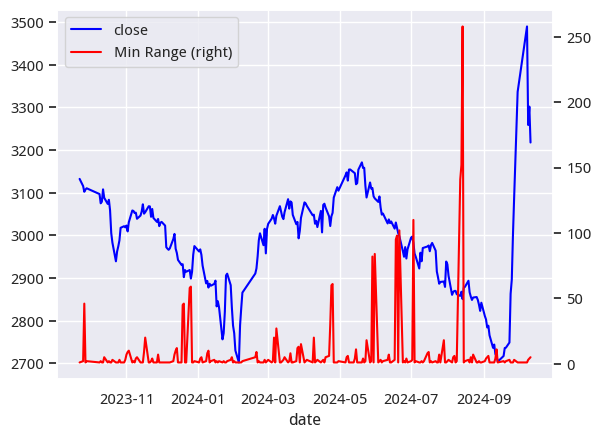
This chart shows astonishing results. Almost every time "low volume" (greater than 50 days) appears, a small rebound follows immediately. However, major rebounds require not just low volume, but also increasing trading volume as capital continuously enters the market.
For example, at the end of August, the Shanghai Index hit its lowest volume in a year, immediately followed by a small rebound. After the rebound failed, other indicators gradually bottomed out and recovered, ultimately leading to the unprecedented surge at the end of September.