Sharpe >4? A-Share Data Standardization Pitfalls

Student Question: I am new to machine learning in trading and have been testing various preprocessing steps. One model suddenly performed far better than any I had previously built, with the only major change being how I standardized the data (Z-score vs. Min-Max vs. L2). I am confused: why does a simple standardization adjustment create such a massive difference? Is there a problem here?

Here is his backtest report:

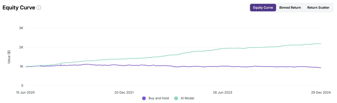
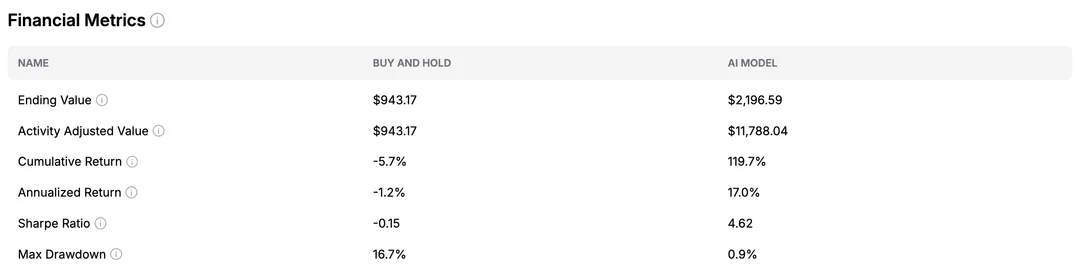
At first glance, this report shows no obvious issues. But as the old Wall Street saying goes: “If it looks too good to be true, it probably is.”

To analyze the problem, we must start from the basics.

A simple rule of thumb: If anyone presents a Sharpe ratio (SR) greater than 4, you can generally assume the strategy has introduced future data (Look-ahead Bias). Why? Because a Sharpe ratio above 4 implies an annualized return exceeding 200%, which is overly idealistic.

## Researching the Relationship Between Sharpe and Annualized Returns

This is a question difficult to answer via direct web searches. Therefore, I will share my research methodology. The core approach uses Monte Carlo simulations to first simulate daily return distributions, and then calculate annualized returns and Sharpe ratios based on these return distributions.

Since return distributions are random, the resulting annualized returns and Sharpe ratios are also random. However, by repeating this process many times, we can obtain a stable distribution of the relationship between the two.

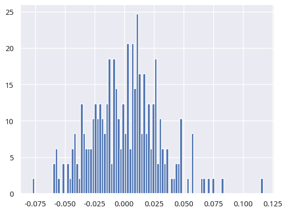
First, we must simulate reasonable daily return distributions based on the asset class. Taking China A-shares as an example, a reasonable distribution is a normal distribution centered at 1e-3 with a scale of 0.03 (optimistic).

This is our simulated daily return distribution:

Based on these simulated return data, we can plot the relationship between annualized returns and Sharpe ratios, as shown below:

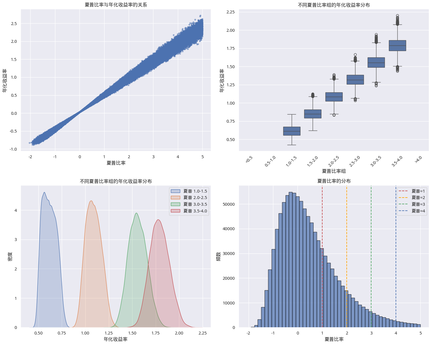
You might argue that a daily return mean of 0 and a scale of 0.02 are more reasonable. In this case (lower volatility), if the strategy’s Sharpe reaches 4, the median annualized return would be 120%, which is still excessively high.

Therefore, when we see a Sharpe ratio greater than 4, we can almost “doubt without hesitation” that the strategy has introduced future data.

How Is Future Data Introduced?

When using statistical methods, we must pay close attention to the time range of the data used. This is one of the most famous traps in quantitative backtesting: Look-ahead Bias.

The student’s issue was that when using Z-score, he standardized the data using the entire backtest period, rather than using data available up to the backtest day.

Mean Reversion with a God’s Eye View

When we use Z-scored data for the entire backtest period, we introduce future data. If the backtest occurs during [start, end], the data distribution in [start, t] is likely inconsistent with the distribution in [start, end].

Imagine you are trading based on Bollinger Bands, which is essentially a dynamic Z-score strategy. What happens if you calculate the Z-score in early 2020 using the global standard deviation derived from the extreme volatility of the US stock market circuit-breaker event in March 2020?

The global standard deviation would be inflated by the extreme volatility during the circuit-breaker period. Consequently, during the normal volatility period before the crash, your model’s calculated Z-score would be smaller than the actual value (because the denominator is larger). This means the model would perceive the market as being in an “abnormally calm” state, or that prices have not deviated far from the mean. During the crash, because you have “foreseen” that this volatility is part of the global distribution, the model might behave unusually calmly during market panic, or even precisely bottom-fish.

This is why the student’s strategy returns became so good—his model had a “God’s eye view,” knowing the answer distribution for the entire exam period in advance.

Why Is Min-Max Normalization More Dangerous?

If we look at the errors caused by Min-Max normalization, the problem becomes easier to understand. This issue is more pronounced in stock and cryptocurrency markets because, theoretically, their trends are not zero-centered symmetric random walks. Stocks grow according to functions related to national GDP growth; cryptocurrencies, being deflationary currencies, grow according to inverse functions of deflation rates.

If these theories are dry and hard to grasp, let us just remember a related conclusion: stock prices can rise to the sky. But if you use data from the [start, end] interval for Min-Max normalization, you are effectively showing the [start, t] interval the max(close[start, end]) that had not yet risen at that time.

If you are using a machine learning model, it usually cannot predict a maximum value that only exists in the [start, end] interval within the [start, t] interval. This normalization effectively tells the model: “The current price is still cheap relative to the highest price seen in the future, buy now!”

The Correct Approach: Rolling Windows

To avoid this self-deception, we must strictly adhere to the Point-in-Time principle. When standardizing at time t, we can only use data prior to t.

The industry standard practice is to use Rolling Windows or Expanding Windows for standardization:

1. Rolling Window: For example, use only the past 250 days of data to calculate the mean and standard deviation for that day’s Z-score standardization. This simulates real-world moving average logic.
2. Expanding Window: Use all data from the start of the backtest to yesterday to calculate statistics.

Although this may cause the model’s performance to “worsen,” this is the real return you can take home. After all, on our path to earning alpha, the first enemy we must defeat is not the market, but our own human nature’s desire to take shortcuts.

Image credit: Dmytro Yarish@unsplash