Monte Carlo: A Brutally Simple Tool for Quant Risk

We often want to know the maximum loss a portfolio might suffer on a future date. One estimation method is Monte Carlo. Although it doesn’t lead in computational performance, it offers the most psychological comfort—after all, it’s a method that walks nearly every possible path to report back on the risks and landscapes encountered along the way.

It looks sophisticated, but it’s essentially brute force. Let’s meet it today.

On May 20, a major event shook the AI industry: Builder.AI declared bankruptcy. Founded in London in 2016 by Indian-born Sachin Dev Duggal, the company had enjoyed immense popularity with its concept of an “AI-driven no-code App development platform,” reaching a valuation of up to $1.7 billion.

However, a 2019 Wall Street Journal report tore away Builder.AI’s false facade. Multiple former employees revealed that many features of the company’s so-called AI platform were actually completed through manual coding by Indian engineers. As time went on, Builder.AI’s fraudulent business model became unsustainable, leading to its eventual exit from the stage on May 20.

Builder.AI excessively promoted its AI capabilities, which was essentially deception and fraud. However, not all “excessive promotion” is unpleasant. Today, we discuss a real, widely used technology. It is brutal and primitive, but romantic scientists have bestowed upon it a high-end name—Monte Carlo Method—making it appear “sophisticated.”

The Monte Carlo method, also known as statistical simulation, is a numerical computation technique that uses random sampling and probability statistics to solve problems in mathematics, physics, engineering, and other fields. Its core idea is to use a large number of random samples to simulate uncertain processes and approximate complex solutions through statistical laws.

The method originated in the 1940s, proposed by mathematicians John von Neumann and Stanisław Ulam while researching neutron diffusion during the Manhattan Project. Since the method relies heavily on random processes, similar to gambling games in Monaco casinos, it was named after Monte Carlo.

Its simplest version is used to calculate $\pi$.

1. Calculating $\pi$ Using Monte Carlo

Assume we have a $2 \times 2$ square. The radius of its inscribed circle is 1, and its area is $\pi$. According to geometric probability, if we randomly throw a point into this square, the probability of it landing in the square (including the inscribed circle) is 1, while the probability of it landing in the inscribed circle is $\pi/4$.

Therefore, if we generate several random pairs $(X, Y)$ in the interval $[-1, 1]$, and for any point $(X, Y)$ satisfying $X^2 + Y^2 < 1$, the point lies inside the inscribed circle. By increasing the number of random pairs, the final ratio of points falling inside the circle represents $\pi$.

We can demonstrate this with the following code:

123456789101112131415161718192021222324252627282930313233import numpy as np
import matplotlib.pyplot as plt

def estimate_pi(n_points=10000, visualization = False):
    # Generate uniformly distributed random points (-1, 1)
    x = np.random.uniform(-1, 1, n_points)
    y = np.random.uniform(-1, 1, n_points)
    
    # Determine if points are inside the circle (x² + y² ≤ 1)
    inside = x**2 + y**2 <= 1
    
    # Calculate pi estimate
    pi_est = 4 * np.mean(inside)
    
    # Visualize results
    if visualization:
        plt.figure(figsize=(6, 6))
        plt.scatter(x[inside], y[inside], s=1, c='blue', label='Inside Circle')
        plt.scatter(x[~inside], y[~inside], s=1, c='red', label='Outside Circle')
        plt.title(f'Estimated π = {pi_est:.6f} (n={n_points})')
        plt.legend()
        plt.show()
    
    return pi_est

# Example run
for n in (100, 10000, 1_000_000):
    pi_estimate = estimate_pi(n)
    print(f"Estimated Pi: {pi_estimate}")
    print(f"Error: {abs(pi_estimate - np.pi):.6f}")

n = 1_000_000
estimate_pi(n, visualization = True)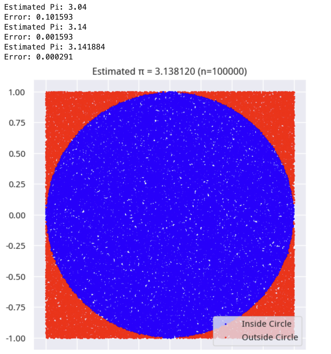

The results show that after more than 1 million random trials, the estimated value of $\pi$ is already very close to the true value. This calculation is simple and brute-force, requiring only 10ms. Although it lacks the precision and performance of the Leibniz series, Ramanujan formula, or Gauss-Legendre algorithm, as an algorithm that doesn’t require much brainpower, it appeals more to someone like me who struggled in school.

2. Calculating VaR Using Monte Carlo

In quantitative finance, the advantage of Monte Carlo is not just simplicity; sometimes, it is irreplaceable. This is due to the unique randomness and unpredictability of financial markets.

VaR (Value at Risk) is a statistical metric used to measure financial risk, representing the maximum potential loss of an asset or portfolio over a specific holding period at a given confidence level.

It can be defined by the following formula:

$$ P(L \geq VaR_\alpha) = 1 - \alpha $$

where $\alpha$ is the confidence level. To explain this formula with an example: if a portfolio’s daily VaR at a 95% confidence level is $1 million, it means that over the next 20 trading days, there may be one day where the loss exceeds $1 million.

As a risk metric, VaR has been endorsed by the Basel Committee. In 1996, the Basel Committee issued the “Supplementary Provisions on Market Risk of the Capital Accord,” allowing banks to use internal VaR models to calculate market risk capital requirements, thereby promoting VaR as a global financial industry standard.

In quantitative trading, we often want to know the maximum loss a portfolio might suffer on a future day, given certain characteristics (such as volatility), to facilitate risk management (such as reducing positions in advance to lower risk). Although there are multiple methods, Monte Carlo, despite not leading in computational performance, often provides the most peace of mind—after all, it is a method that walks nearly every possible path to tell you about the risks encountered along the way.

1234567891011121314151617181920212223242526272829303132import numpy as np
import matplotlib.pyplot as plt
from scipy.stats import norm

# Portfolio parameters
initial_stock_price = 100    # Initial stock price
stock_volatility = 0.2       # Annualized stock volatility
risk_free_rate = 0.05        # Risk-free rate
option_strike = 105          # Call option strike price
option_maturity = 0.5        # Option remaining maturity (years)
num_options = -10            # Number of short option positions (negative indicates selling)
num_shares = 1000            # Number of long shares
portfolio_value = num_shares * initial_stock_price  # Initial portfolio value

# Simulation parameters
num_simulations = 10000      # Number of simulations
time_horizon = 10/252        # Time span of 10 trading days (annualized)
dt = 1/252                   # Time step

# Black-Scholes option pricing function
def black_scholes_call(S, K, r, sigma, T):
    d1 = (np.log(S/K) + (r + 0.5*sigma**2)*T) / (sigma*np.sqrt(T))
    d2 = d1 - sigma*np.sqrt(T)
    return S * norm.cdf(d1) - K * np.exp(-r*T) * norm.cdf(d2)

# Calculate current option value
current_option_value = black_scholes_call(initial_stock_price, option_strike, 
                                          risk_free_rate, stock_volatility, option_maturity)

# Calculate current portfolio value
current_portfolio_value = num_shares * initial_stock_price + num_options * current_option_value * 100  # Option contract multiplier 100
print(f"Current Portfolio Value: ${current_portfolio_value:.2f}")

This gives us a random portfolio with a current value of $95,418.32.

Next, assume we are concerned with the returns and risks of holding this portfolio for 10 days. We don’t know how the price movements of each asset will evolve, but we can “guess” as follows:

12345678910111213141516171819202122232425# Generate random return paths
np.random.seed(42)  # Set random seed to ensure reproducibility
daily_returns = np.random.normal((risk_free_rate * dt), 
                                (stock_volatility * np.sqrt(dt)), 
                                (num_simulations, int(time_horizon/dt)))

# Calculate cumulative returns and future stock prices
cumulative_returns = np.cumprod(1 + daily_returns, axis=1)
future_stock_prices = initial_stock_price * cumulative_returns[:, -1]

# Calculate future option maturity
future_option_maturity = option_maturity - time_horizon

# Calculate future option values (considering time decay and stock price changes)
future_option_values = np.array([black_scholes_call(S, option_strike, risk_free_rate, 
                                                    stock_volatility, future_option_maturity)
                                for S in future_stock_prices])

# Calculate future portfolio value
future_portfolio_values = num_shares * future_stock_prices + num_options * future_option_values * 100

# Calculate portfolio value changes (loss is negative return)
portfolio_changes = future_portfolio_values - current_portfolio_value
losses = -portfolio_changes  # Convert negative returns to positive losses
losses

At this point, we have obtained 10,000 possible outcomes for the portfolio’s returns and losses 10 days later.

Next, we can use a small statistical trick to calculate VaR at different confidence levels:

123456789101112confidence_levels = [0.95, 0.99, 0.999]
var_values = {}

for cl in confidence_levels:
    var = np.percentile(losses, (1 - cl) * 100)
    var_values[cl] = var
    print(f"{cl*100:.1f}% VaR: ${var:.2f}")

# Calculate ES (Expected Shortfall) at 95% confidence level
var_95 = var_values[0.95]
es_95 = np.mean(losses[losses >= var_95])
print(f"95% ES (Expected Shortfall): ${es_95:.2f}")

95.0% VaR: $-3446.95 99.0% VaR: $-4387.73 99.9% VaR: $-5235.53 95% ES (Expected Shortfall): $14.24

This portfolio is indeed a money-losing machine. It has a 95% probability of losing $-3,446.95. However, the 95% ES data tells us that even if a loss occurs, in the case of losses exceeding $-3,446.95, you would on average only need to lose an additional $14.24.

3. Estimating Maximum Drawdown Based on Sharpe Ratio

Assume you have an excellent strategy with a Sharpe ratio of 2 during drawdowns; generally, this is a quite good strategy. However, you also know that backtests are never identical to live trading, so you want to know:

Obviously, we cannot simply compare the current drawdown with the maximum drawdown from backtests. The latter is a scalar with no statistical significance. However, in live trading, maximum drawdown is a more sensitive indicator and a greater concern for investors than the Sharpe ratio. We must answer this question: Does the current maximum drawdown exceed the range allowed by the Sharpe ratio, implying that the strategy has failed?

We discussed this issue in “Kuang Ti’s 24 Quantitative Lessons,” using the Monte Carlo method. Through 50 million simulations under different Sharpe indicators, we derived the following answers for reference in live trading:

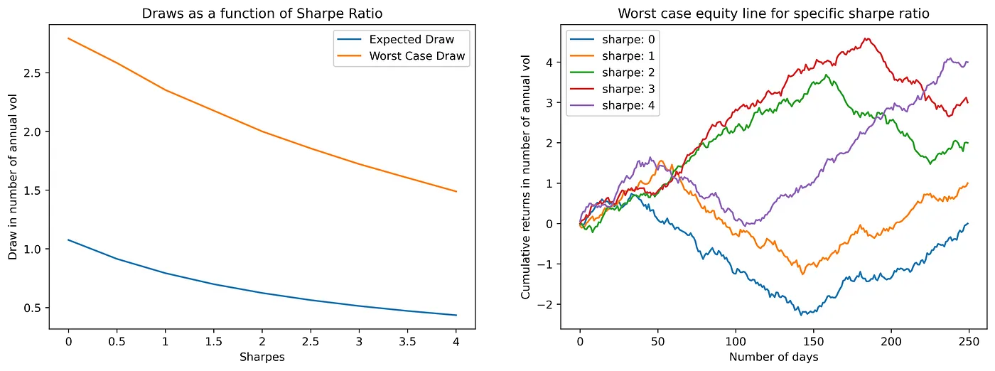
In this chart, blue represents normal conditions, and yellow represents the worst-case scenario. The X-axis is the Sharpe ratio. What is the Y-axis? It is not the maximum drawdown itself, but the ratio of maximum drawdown to annualized volatility, which is more scientific.

Taking the left chart as an example, when the Sharpe ratio is 1.5, if the maximum drawdown is 0.7 times the annualized volatility, the strategy is still in a normal state. However, you might consider stopping the strategy execution if the maximum drawdown exceeds 0.7 times the annualized volatility. If the maximum drawdown is 2.18 times the annualized volatility, the strategy is in the worst state. If already in this state, you might expect a small rebound before exiting the strategy.