How to Normalize Factors for Deep Learning Strategies

How should normalization be implemented in a deep-learning-based quant strategy? This article first distinguishes between normalization, standardization, and regularization, then analyzes common mistakes when using min-max, sine, sigmoid and other normalization functions in quant research, explains how to build a good normalization function, and closes with several factor-normalization examples.

Normalization, Standardization, and Regularization

Normalization, standardization, and regularization are similar but distinct concepts in machine learning and deep learning.

Normalization generally means mapping a data distribution into the interval [0,1]. Most of us first encountered the idea in statistics, where the main method is min-max scaling, but in deep learning the toolkit goes far beyond that, including tanh, sigmoid, sine, and more. The min-max normalization formula is:

$$ X' = \frac{X - min(x)}{max(X) - min(X)} $$

Not every function that maps values into [0,1] qualifies as a normalization function. A normalization function must preserve the ordering of the data. For example, if inputs $[x_0, x_1]$ map to $[y_0, y_1]$, and $x_0 >= x_1$, then $y_0 >= y_1$ must also hold. We can call this the monotonicity principle. For this reason, functions like sine are rarely used in deep learning — though not absolutely never. What makes a good normalization function? We will return to that below.

In practice, we can use sklearn.preprocessing.MinMaxScaler for this transformation.

Standardization usually refers to the following transformation:

$$ z = \frac{X - \mu}{\sigma} $$

that is, z-scoring. After standardization, z follows a $N(0,1)$ normal distribution. In practice, we can use sklearn.preprocessing.StandardScaler (or scale()) for this.

Normalization and standardization are actually quite different. After normalization, values fall in [0,1] (or [-1,1]). By removing units, physical quantities with different dimensions can then be optimized with the same learning rate in gradient-based deep learning. A standardized dataset, by contrast, has no bounded range, so it still carries units. Different factors remain dimensionally inconsistent after standardization, so they cannot be trained together. Moreover, standardization is only meaningful if the dataset itself is approximately normally distributed.

Regularization here means dividing the standardized data by its norm, squeezing the data into the [-1,1] interval. The regularized result is unit-free and suitable for deep learning. The formula is:

$$ X' = \frac{X}{||X||} $$

In sklearn, this is implemented as sklearn.preprocessing.Normalizer.

For some machine learning algorithms, such as decision trees and boosting methods, none of these three transforms is necessary, because those algorithms are insensitive to units.

In deep learning, however, weight optimization involves the learning rate, so all input vectors — factors, in quant terms — must share a consistent scale. We therefore must apply normalization or regularization. Standardization alone is of little use.

Deep learning offers many normalization methods, far beyond the statistical min-max scaler. Which one to use depends on the data distribution and the problem at hand, so sigmoid, tanh, sine — the latter was first used in NMT — min-max, and others all see use.

Common Normalization Functions

Min-Max Scaling

In a deep-learning-based quant strategy, never apply min-max scaling directly to a raw stock price — or to any first-order linear transform of price — and treat it as a factor. In many other domains min-max normalization works because the data is bounded. Human height, for example, is roughly 20cm to 250cm — a well-defined range. Stock prices have only a lower bound, with no upper bound. Take Vanke, for example: on a backward-adjusted basis, its price reached 3,700 yuan in 2018. If you had built a factor from pre-2000 prices with min-max scaling, your forecasts could never have exceeded the historical high known at the time.

Returns, RSI and similar indicators are much better suited to min-max scaling. Note that they are second-order functions of price.

Sigmoid and Tanh

These two functions behave almost identically, but in deep learning we use sigmoid more often because its derivative is cheaper to compute.

$$ S = \frac{1}{1 + e^{-x}} $$

The derivative of the sigmoid is:

$$ dS = S * (1 - S) $$

so the computation can reuse the original function value, which makes it faster.

Their transformation curves look like this:

Sine

In general, we do not use the sine function for normalization because its values are periodic. But this is not absolute. Google's early NMT models used sine extensively for normalization, precisely because it captures the periodicity in the distance between two related morphemes. Although sine-based normalization is rarely reported in deep-learning quant strategies, given the cyclicality of the economy and of trading behavior, periodic normalization functions should have a role to play in factor extraction.

Z-Score and Regularization

As discussed above, the z-score method cannot remove units and is therefore generally unsuitable for deep learning. Regularization can compress data into the [0-1] interval, but as with min-max, we cannot feed price transforms directly as factors. The same caveat likely applies to other methods.

Some argue that we cannot use z-score transforms because stock fluctuations are not normally distributed, but the main issue is really units. Whether the data is normal matters more for whether — and how — we can perform statistical inference. In addition, with non-normal data, data points tend to cluster together instead of spreading evenly.

This raises the question of how to evaluate a normalization function — what makes a good one.

What Makes a Good Normalization Function

In a quant strategy, a good normalization function must first satisfy the monotonicity principle, and second, give the best response sensitivity to the most frequently occurring data points. Resolution also matters.

Note that some functions are monotonic mathematically but violate monotonicity in computer implementations because of floating-point error.

For example, which is larger, sigmoid(13) or sigmoid(26)? Mathematically, since $26 > 13$, $sigmoid(26) > sigmoid(13)$ should hold. In practice, however, the code below shows the two values are equal:

123456import numpy as np

def sigmoid(x):
    return 1/(1 + np.exp(-x))

assert sigmoid(13) - sigmoid(26) < 1e-7

1e-7 is the finest precision representable by 32-bit floats. In deep learning, weight matrices are typically 32-bit, and 16-bit weights are now common as well.

sigmoid(13) equals sigmoid(26)! That breaks the monotonicity principle.

The other issue is response sensitivity. Why do we apply z-score transforms? To map the most frequent data range to the region around zero, where response sensitivity is highest.

As the sigmoid vs. tanh comparison shows, for sigmoid, inputs in the [-5,5] range produce sigmoid values with good sensitivity to x; beyond that range the response saturates. Such saturation means we must use a smaller learning rate to tune the model well.

So we generally do not use sigmoid directly, but a transformed version of it:

1234567def scaled_sigmoid(x, start, end):
    """当`x`落在`[start,end]`区间时，函数值为[0,1]且在该区间有较好的响应灵敏度
    """
    n = np.abs(start - end)

    score = 2/(1 + np.exp(-np.log(40_000)*(x - start - n)/n + np.log(5e-3)))
    return score/2

The chart below shows that when data is concentrated in different [start, end] intervals, the transformed sigmoid still gives the best response sensitivity around the center of the distribution — which is also why we do z-score transforms.

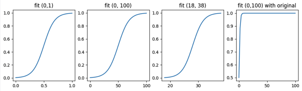
In subplot 1, we give data in [0,1] the best response sensitivity. In subplot 2, if data often sits around 50 and fluctuates by plus or minus 50, it still gets the best sensitivity. Subplot 4 shows the raw sigmoid over [0,100].

Factor Normalization Examples

Post-Limit-Up Consolidation Factor

A stock hitting the price limit is a sign of strength — try it yourself and see how hard it is to keep a stock locked limit-up from 10:00 a.m. without it opening. Since you cannot buy on the limit-up day itself, but the stock may consolidate afterward, there may be an opportunity to enter at a lower level. We want to know roughly how many days after the limit-up gives the highest win rate.

This is a case where sine can be used for normalization. Days since the limit-up has no monotonic meaning — a longer consolidation does not imply a higher probability of rallying. Instead, it may follow some kind of cycle.

Low-Volume Factor

If a stock — or the market on a given day — prints extremely low volume, sentiment has frozen to the extreme and the decline is exhausted. As the old saying goes, extremely low volume marks the bottom.

We can describe low volume by how many days (n) the current volume is the minimum over. Clearly, a larger value is better. But it cannot grow without bound — otherwise the adage would not hold.

We can run the statistics, pick a reasonable interval, and use the scaled_sigmoid above to extract a factor for deep learning. The lower bound of that interval should probably start at least at 30.

Probability Factor

Once converted into probabilities, some data naturally lives in [0,1]. So when we have no clear normalization idea, we can estimate the empirical distribution function to obtain empirical CDF/PPF functions, and then use the probability associated with each observation as a factor for deep learning.

If concepts in this article such as floating-point error, the role of normalization functions, or CDF/PPF are unfamiliar, you may need to study quant courses more systematically. This post is adapted from our course materials — feel free to join us!