Probability Theory Axiomatized: From Gambling to Kolmogorov

In the previous article, we solved problems using elementary probability methods. This approach requires us to "count" the total number of sample points and the number of elementary events contained within specific events. The probability is the ratio of these two numbers.

If the elementary events are uncountable, we can use geometric probability, converting counting into the calculation of ratios of "length, area, or volume."

However, these methods require high levels of skill and often impose conditions such as finite events or uniform distribution of elementary events within a geometric region. This is akin to many elementary school math olympiad problems: while the problems themselves are not difficult to solve, restricting the solution to elementary mathematics raises the bar for "technique." You must rely on keen mathematical intuition and complex techniques to map simple concepts from high-dimensional spaces into understandable, solvable objects in low-dimensional spaces. Moreover, our description of the problem-solving process relies heavily on ambiguous natural language rather than precise mathematical language, which casts doubt on the correctness of our answers.

In the previous article, we already felt this constraint. The solution path seemed simple, but in reality, to find the correct answer, I had to revise my approach multiple times. Almost every version was mixed with poorly defined natural language descriptions, particularly regarding why we needed to eliminate duplicates. It felt like we had explained it, yet not quite explained it, resembling a "guess-the-answer" approach where we intuitively derive a general term and then use the first few terms to justify the formula. It was only when I finally found the precise mathematical description—that $n$ points belonging to the same semicircle is equivalent to the maximum angle spanned by those $n$ points being less than $\pi$—that I could precisely eliminate the double-counted events.

So why not master more precise mathematical languages and more effective mathematical tools to simplify the complexity of our thinking?

What is Probability?

Humanity’s earliest recognition of probability problems stemmed from gambling. For instance, in 1654, the French nobleman and gambler Chevalier de Méré posed a classic problem to the mathematician Blaise Pascal: two people agree to gamble, with the first to win 5 rounds taking the prize. If the game is interrupted, how should the stakes be fairly distributed based on the current score (e.g., one player has won 4 rounds and the other 2)?

The core of this problem is calculating the "probability of winning the remaining rounds." Pascal and Fermi communicated via letters, systematically calculating this "expected probability" using combinatorial mathematics for the first time, laying the early foundation for probability theory.

From Gambling to Classical Probability

In gambling, many scenarios feature "a finite number of equally likely outcomes," and gamblers need to calculate the ratio of "favorable outcomes" to "total outcomes." Mathematicians distilled this ratio into the definition of classical probability.

Its core viewpoint is that a random event consists of several "equally likely," mutually independent (mutually exclusive) elementary events. By counting the "elementary events" that constitute an "event," we can determine the probability of that "event."

For example, when tossing a fair coin, the possible outcomes are heads (denoted as H) and tails (denoted as T), totaling 2 elementary events. These two elementary events are equally likely, meaning each has a probability of $1/2$. Furthermore, in a single experiment, once one elementary event occurs, no other elementary event can occur. Thus, these 2 results constitute 2 "elementary events."

Under the above premises, consider:

The event requested in the problem is composed of elementary events. The combinations of all possible elementary events are:

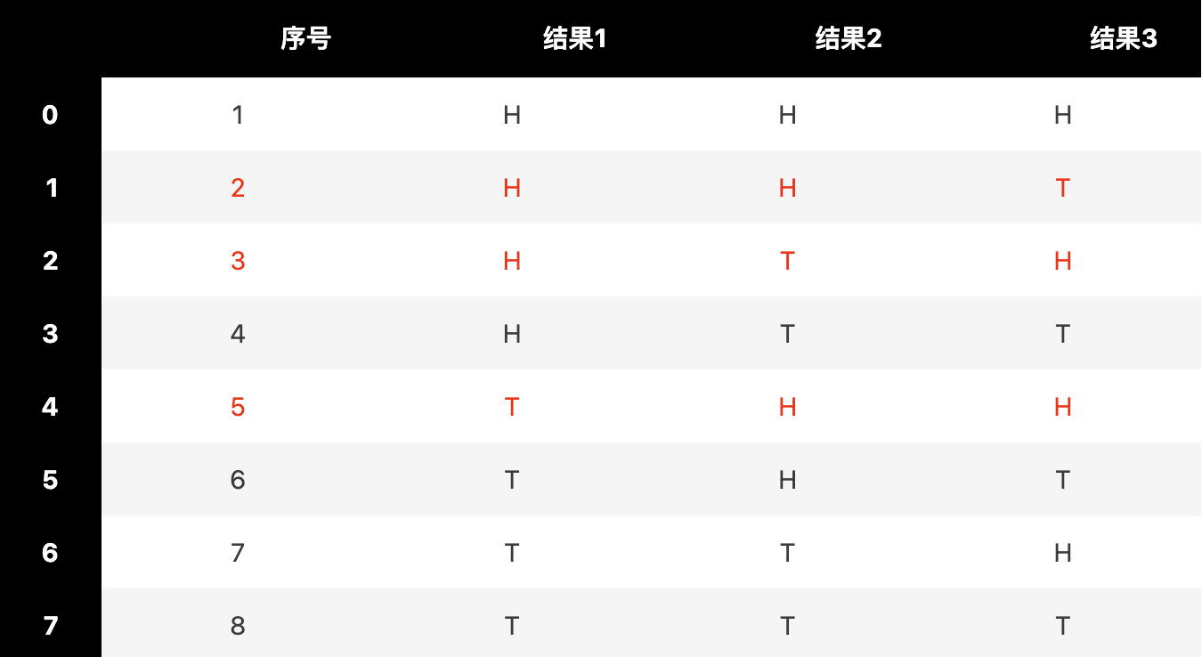
Among these, there are exactly three events with heads appearing exactly twice: sequences 2, 3, and 5. From this, we summarize the formula for classical probability:

$$ P(A) = \frac{\text{Number of elementary events contained in event } A}{\text{Total number of all possible elementary events}} $$

When the problem scale is large, the enumeration method above encounters computational difficulties. In such cases, we may apply classic formulas. For example, the problem above can be solved using the general formula for the binomial distribution:

However, we find that concepts such as "elementary events" and "events" are difficult to distinguish in the above problem-solving process. For instance, in the dice-rolling example, if we ask for the probability of rolling a 1 in a single throw, the elementary event and the event are completely identical.

Furthermore, counting elementary events can sometimes be confused with the concept of frequency. For example, in the dice-rolling scenario, if you casually throw a die three times and a 1 appears twice, why is the probability of rolling a 1 not calculated as 2 (the number of times 1 appeared) divided by 3 (the number of throws)? The reason is that elementary events constituting an event is a thought experiment, independent of the actual number of throws.

This indicates that classical probability theory, even in its area of expertise—discrete probability—often suffers from confusion and ambiguity, necessitating further expansion and axiomatization of related concepts.

Additionally, classical probability cannot resolve the following issue:

Classical probability requires elementary events to be finite and countable. In the above problem, the elementary events are infinite because there are infinitely many points in the interval [0, 1].

When elementary events are infinite but possess geometric significance, we can use geometric probability to solve the problem.

From Finite to Infinite: The Proposal of Geometric Probability

The basic model of geometric probability is:

1. All possible trial results (sample space) correspond to a measurable geometric region $\Omega$ (such as a line segment, planar region, or spatial solid);
2. The occurrence of each elementary event corresponds to a point within region $\Omega$, and the point is uniformly distributed within the region (i.e., "equally likely" means the probability of the point being at any position within the region is equal).

At this point, we can express the probability using the following formula:

Based on the above definition, we can calculate the answer to Problem 2 as $(0.5 - 0.2)/(1-0) = 0.3$.

In this definition, length, area, and volume are specific manifestations of "measure." In modern mathematics, this concept is rigorously formalized as "Lebesgue Measure" (proposed in 1901). It generalizes our intuitive understanding of length, area, and volume to more complex sets, providing a solid theoretical foundation for geometric probability and laying the groundwork for the axiomatization of probability.

In Lebesgue measure, the measure of a simple interval $[a,b]$ is $b-a$, which is exactly the same as the length we usually refer to. For a single point, its Lebesgue measure is 0 because a point has no "length."

The core premise of geometric probability is "uniform distribution," meaning points are uniformly distributed within the sample space, and probability is proportional to the region's measure, requiring a way to measure the region. Therefore, there are still many probability problems that geometric probability cannot solve, such as:

The lifespan of a light bulb follows an exponential distribution. How do we calculate the probability that the lifespan exceeds 1000 hours? It is difficult to calculate this directly via the "ratio of time interval lengths."

However, the emergence of geometric probability has laid the foundation for modern probability theory, as it is easy to link geometric measures with integrals. Thus, in 1933, mathematician Andrey Kolmogorov, summarizing early models such as classical and geometric probability, proposed the axiomatic definition of probability in 1933, abstracting probability from specific scenarios into a strict mathematical theory.

Kolmogorov Axioms

Let the sample space of a random experiment be $\Omega$. For each event A (i.e., $A \subseteq \Omega$), assign a real number $P(A)$. If $P(A)$ satisfies the following three axioms, then $P(A)$ is called the probability of event A:

• Axiom 1 (Non-negativity): For any event A, $P(A) \geq 0$;
• Axiom 2 (Normalization): The sample space $\Omega$, as a certain event, has a probability of 1, i.e., $P(\Omega) = 1$;
• Axiom 3 (Additivity): If events $A_1, A_2, \dots$ are mutually exclusive (i.e., any two events share no common sample points), then $P(A_1 \cup A_2 \cup \dots) = P(A_1) + P(A_2) + \dots$.

Although this definition is abstract and differs significantly from the intuitive impression we form when first learning probability, and even the probability $P(A)$ itself may not directly represent the likelihood of event A occurring,

it is precisely this abstract definition that allows continuous random variables and discrete random variables (discrete events) to be described uniformly within the same framework. The only difference between them lies in the method of calculating probability: in the discrete case, we sum the probabilities of each event, while in the continuous case, we must use integration. In fact, integration can be viewed as a process of "continuous summation" or "finding area," so both types of problems are essentially unified.

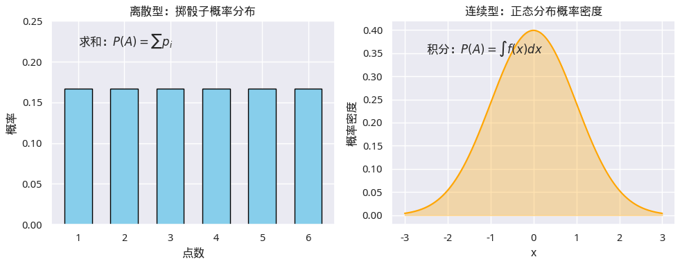
However, as practical problems become more complex, relying solely on intuition or simple counting methods is no longer sufficient. Therefore, we need more powerful mathematical tools to systematically characterize and calculate probabilities. Thus, through axiomatization, the definition of probability no longer depends on specific scenarios or intuitive assumptions but is built upon a clear mathematical foundation. It can handle both finite, discrete problems and be generalized to infinite, continuous cases. Based on Kolmogorov’s axioms, we have entered the modern era, where the mathematical tools established since Newton’s time—integrals and derivatives—can finally be put to use.