Quant Interview Trap: Probability of Random Points on a Circle

It is often asked: What mathematical foundation is required for quantitative trading?

The mathematical prerequisites vary significantly across different quant research domains. Generally, the hierarchy of mathematical depth is: Options > High-Frequency > Futures > Mid-to-Low Frequency Equity.

Today, we discuss the mathematical foundations required for each domain and use a classic quantitative interview question (from the "Green Book") to illustrate the concepts institutions may test, ranging from elementary to intermediate probability theory.

This article is lengthy and will be published in two parts.

Mid-to-Low Frequency Equity Quant

We need to master basic probability theory and mathematical statistics. This includes understanding the distribution characteristics of statistical variables (mean, variance, quantiles); grasping hypothesis testing (how to determine significance); linear regression; and correlation analysis.

Understanding the distribution characteristics of statistical variables is fundamental and is used constantly in quant finance. For instance, to evaluate which of two quantitative strategies is better, the most basic metric is its daily average return. However, with basic statistical knowledge, it becomes clear that identical means do not imply that two random variables are identical. Therefore, it is easy to understand why geometric returns are used instead of daily average returns to judge a strategy's profitability. A solid statistical foundation helps us expand our conceptual toolkit and know which concept to apply in which context. This is just one example.

In multi-factor strategies, we extensively use linear regression to determine factor weights (regressing factor weights against forward returns). Additionally, in multi-factor strategies, we often use orthogonalization to neutralize the impact of correlated factors, typically by obtaining orthogonalized factors via linear regression residuals.

When assessing factor validity, we involve significance testing theories, requiring an understanding of p-values and t-values.

Correlation analysis is also used in factor mining. We use correlation tests (Pearson or Spearman) to determine if a factor correlates with future returns.

Of course, we must also master the normal distribution, understanding its distribution properties, key quantiles ($\mu + \sigma, \mu + 2\sigma, \mu + 3\sigma$), its underlying principles, and its applicable scope.

Regarding linear algebra and calculus, if you are not engaging with machine learning, deep mastery is not strictly necessary. You can leverage existing Python libraries when needed. However, it is recommended to deeply master PDFs (Probability Density Functions) and CDFs (Cumulative Distribution Functions). Once mastered, understanding elementary probability problems becomes as simple as solving primary school arithmetic after mastering calculus.

These topics are largely covered in Quantitative Trading 24 Lessons.

Futures Quant

This domain requires mastery of time series analysis, such as GARCH models and cointegration tests. For example, in a rebar futures calendar spread arbitrage strategy, we must confirm that the prices of near-month and far-month contracts exhibit a long-term equilibrium relationship before establishing an arbitrage basis. This requires a deep understanding of the significance of stationary time series, the concept of cointegration, and how to perform cointegration tests.

High-Frequency Quant

High-frequency quant involves algorithms for order flow modeling, short-term price prediction, and optimal order execution strategies, imposing higher demands on probability and mathematical statistics.

For instance, in order flow direction prediction, conditional probability and extreme value theory are often used. When modeling price distributions, kernel density estimation (KDE) is employed and validated through hypothesis testing. In order arrival modeling, Poisson processes may be used; for short-term price state transition prediction, Markov chains might be applied. These are contents of stochastic processes, representing the advanced stage of probability theory.

Additionally, optimization theory (convex optimization) is frequently involved. For example, the optimal quoting strategy for high-frequency market makers is a convex optimization problem, and dynamic programming algorithms may be used for optimal order timing selection.

Of course, there is another path: deeply mastering machine learning theory and frameworks allows one to "force" solutions with raw computational power, potentially lowering the strict mathematical requirements mentioned above.

Since high-frequency quant demands extreme speed, many computations require matrix operations for efficiency. Thus, there are also requirements for linear algebra.

Options Quant

The core issues in options quant are derivative pricing, volatility modeling, and risk hedging (Greeks calculation). This domain has the highest mathematical demands, generally requiring mastery of Brownian motion, Itô's lemma, stochastic differential equations, partial differential equations, higher-order derivatives (for Greeks calculation), and complex analysis.

In summary, options are 'designed' derivatives, demanding extreme mathematical depth and derivation capabilities. They represent the highest bar for mathematical ability in the quant field.

So, to what depth do institutions test probability and statistics when hiring? We will use an institutional interview question as an example to illustrate the required level of probability and statistics mastery, excluding options trading scenarios.

We will explain this in detail. The solution will be split into two parts, step-by-step covering elementary probability solutions and solutions using integration, PDFs, and other tools.

The Multi-Point Semi-Circle Problem

This is a problem from the "Green Book": What is the probability that $n$ randomly selected points on a circle all lie within the same semi-circle?

This problem can be solved using elementary probability knowledge or using tools like integration and PDFs. Here, we provide both solutions, particularly using the latter to connect related concepts.

Elementary Probability Method

Elementary probability focuses on intuitive understanding and basic calculations, avoiding overly complex mathematical tools. However, with clever构思, it can solve complex probability problems. This problem is an example.

We first introduce the following figure:

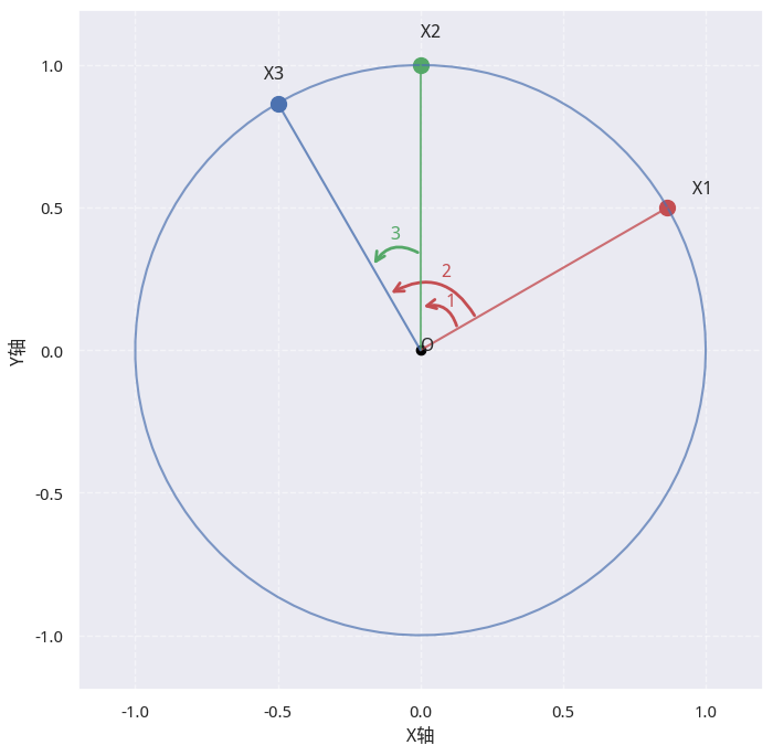
In the figure, the maximum angle that three points can form is one of $\angle X_1OX_2$, $\angle X_1OX_3$, or $\angle X_3OX_2$ (in this figure, $\angle X_1OX_3$). Simultaneously, there exists a symmetric angle, $\angle X_3OX_1$, which essentially refers to the same arc.

Assume we denote the maximum angle that can be formed by $n$ points as $\alpha$. When $\alpha \le \pi$, the problem's condition is satisfied. Therefore, counting the event 'n points are in the same semi-circle' (event $a$) is actually equivalent to checking if 'the maximum angle formed by n points $\alpha \le \pi$' holds (event $b$). The two are identical: counting event $b$ is equivalent to counting event $a$.

Now, we officially begin the discussion.

Step 1: Assume we randomly select one point from the $n$ points to fix (denote this point as $X_1$). Based on this, calculate the probability of subsequent events satisfying the problem's requirements, denoted as $P_{X_1}$. According to the law of total probability:

$$ \begin{align} P &= P_{X_1} + P_{X_2} + ... + P_{X_n} \ &= P_{X_i} * n \end{align} $$

Since each point is equal in random selection, each $P_{X_i}$ should be consistent in probability. Next, we discuss $P_{X_i}$.

Step 2: Assume we select the $i$-th point as the fixed point. The probability that the remaining $n-1$ points all fall to the right of $X_i$ (i.e., to the right of line $X_iO$) is $\frac{1}{2^{n-1}}$. This is because line $X_iO$ divides the circle into two equal halves, and the point falling into any part is an independent random event with a probability of $\frac{1}{2}$. Therefore, we obtain the probability $P_A$ at this time:

$$ P_{X_i} = P_{X_iL} + P_{X_iR} = \frac{1}{2^{n-2}} $$

Here, $P_{X_iL}$ is the event (remaining points all fall to the left of $X_iO$, and the angle <$\pi$). $P_{X_iR}$ is the event (remaining points all fall to the right of $X_iO$, and the angle <$\pi$).

Thus, the total probability of all events is now:

$$ \begin{align} P &= n \times P_{X_i} \ &= n \times \frac{1}{2^{n-2}} \end{align} $$

Below, we verify the correctness of this conclusion. When $n = 2$, we get a probability $P = 2$, which is obviously incorrect. Why?

The issue is that the law of total probability requires us to count only mutually exclusive events. However, in the previous counting, events that appear different but are actually the same were counted multiple times.

Let us discuss starting with two points $X_1, X_2$. At this time, we have:

$$ \begin{align} P = P_{X_1} + P_{X_2} \end{align} $$

Since any two points on the same circle are always in the same semi-circle (if not on the left, then on the right), the probability of any selected point starting the count, with the other point falling into that point's semi-circle, is 1. This is certain.

The problem is that the maximum angle between two points, $\angle X_1OX_2$ and $\angle X_2OX_1$, is actually the same event, yet we counted it twice. Specifically, when we fix $X_1$, we count the event corresponding to angle $\angle X_1OX_2$ when $X_2$ falls into the right half-side of $X_1$; and when we fix $X_2$, we count the event corresponding to angle $\angle X_2OX_1$ when $X_1$ falls into the left half-side of $X_2$. However, these are actually the same event corresponding to $\angle X_1OX_2$. Therefore, we should divide the result of equation 5 by 2.

Generalizing this, for any maximum angle $\angle X_iOX_j$ that satisfies the condition, we count the same event twice: once when fixing $X_i$ and once when fixing $X_j$. Therefore, for any $n$ points, we should divide the probability obtained in equation 4 by 2. Thus, we obtain the final formula:

$$ \begin{align} P &= n \times P_{X_i} / 2 \ &= n \times \frac{1}{2^{n-2}} / 2 \ &= n \times \frac{1}{2^{n-1}} \end{align} $$

Within the realm of elementary probability, we need to understand some primary distributions (such as uniform distribution, Bernoulli distribution), independent events, and other principles, and cleverly use the idea of geometric probability to solve problems.

In the next article, we will fully restore key concepts such as probability, probability density functions, distribution functions, and expectations, as well as how mathematical concepts evolve from concrete to abstract.