Why Do We Need Causal Convolution?

Market volatility is incredibly complex. In the early stages of writing quantitative strategies, we almost all fall into an obsession with “perfect parameters,” attempting to find certainty in the market using the simplest indicators.

Whether it’s the Moving Average (MA), MACD, or Bollinger Bands, we endlessly enumerate values in the backtest engine, trying to find the number that perfectly fits history: Should the moving average be 20 days or 30 days?

However, when we deploy that “optimal parameter” found via grid search into live trading, the results often fall significantly short.

This is because the market is alive. Short-term博弈, medium-term trends, and long-term macroeconomic cycles mix in different proportions every day. Fixed parameters simply cannot handle this chaotic variation.

In this article, we discuss how to use Causal Convolution to let the model “refine” a set of weights directly from the K-line data.

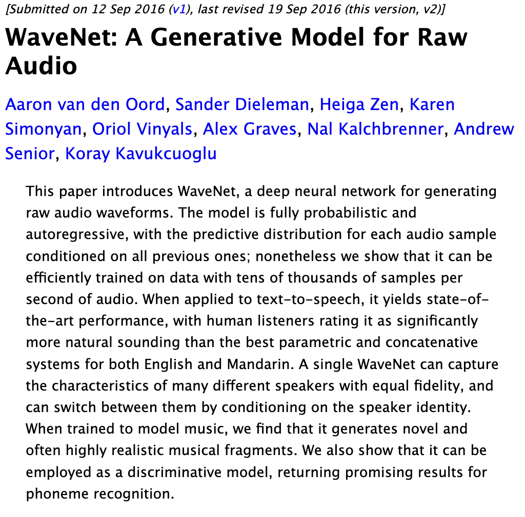
Causal convolution originates from a 2016 DeepMind paper, WaveNet: A Generative Model for Raw Audio.

To solve the problem of “not peeking at future data” in speech generation, Van Den Oord et al. transformed standard convolution into causal convolution (combined with dilated convolution), ensuring the model relies only on historical information to generate the next audio sample.

Deconstructing the Moving Average: It’s Human Arrogance to Frame an Uncertain Market with a Perfect Exponential Curve

To understand causal convolution, let’s take a different perspective and re-examine the moving average we know best.

Take MA5, for example. It sums the closing prices of the past 5 days and divides by 5.

In the context of digital signal processing, this is a sliding filter with equal weights of 1/5. It is very democratic; data from the past five days is treated equally.

But anyone with trading experience knows: does a large bearish candle that just occurred yesterday have the same guiding significance for today’s trend as a doji star from five days ago?

Obviously not. More recent data contains more core information.

This is why quantitative pioneers introduced the EMA (Exponential Moving Average). EMA assumes that history always plays a role, so it never discards any K-line; however, it dictates that the value of information must decay exponentially over time.

But here, we are making a mistake of “human arrogance”: Why must the decay of market sentiment follow a perfect, smooth exponential curve?

If the Federal Reserve unexpectedly raised interest rates three days ago, or if the Non-Farm Payrolls data was a massive surprise, the weight of the K-line on that day should logically be much larger than that of a calm yesterday. The EMA, with its hardcoded mathematical rules, simply cannot handle such “jumps” in weight allocation.

Mathematically, both MA and EMA are essentially calculating a convolution: $$ y_t = \sum_{i=0}^{k-1} w_i \cdot x_{t-i} $$ For MA, the weights $w_i$ are all $\frac{1}{k}$; for EMA, the weights $w_i$ are fixed values decaying exponentially as $\alpha(1-\alpha)^i$.

The question is: Why must the decay of market sentiment be an exponential curve? If the Fed unexpectedly raised rates three days ago, the weight of that day should logically be much larger than yesterday’s. The EMA’s hardcoded rules cannot handle such “jumps.”

Causal convolution uses the same formula above, but instead of having the human brain decide on the decay curve, it hands the weights $w_i$ over to a neural network, allowing them to be learned through backpropagation.

Why Emphasize “Causal”?

The word “causal” in causal convolution is designed to prevent the most common problem in backtesting: Data Leakage (Look-Ahead Bias).

Standard CNNs are successful in image processing because looking at global information when identifying an image is fine.

But if you apply standard convolution directly to K-lines, it will convolve in data from $t+1$, $t+2$, etc., effectively seeing tomorrow’s closing price while making today’s decision.

When a model uses a standard convolution kernel to calculate features for today ($t$), the sliding window inevitably convolves in data from tomorrow ($t+1$) or even the day after.

This is equivalent to the model having already “seen” tomorrow’s closing price while making a trading decision today.

Models trained with such structures often show惊人的 Sharpe ratios during backtesting but collapse quickly in live trading.

As Marcos Lopez de Prado said: “In finance, the hardest problem is never prediction, but verifying whether you’ve cheated.”

To completely eliminate this “cheating” in the network structure, we need to introduce the constraint of “causality.”

The core principle of causal convolution is very clear: today’s output can only depend on today’s and previous historical inputs; it must never cross the boundary.

In the standard convolution formula $y_t = \sum_{i=-k}^{k} w_i \cdot x_{t-i}$, negative $i$ represents extracting future data. Causal convolution forcibly modifies the formula to: $$ y_t = \sum_{i=0}^{k-1} w_i \cdot x_{t-i} $$ Completely cutting off the inflow of future information such as $x_{t+1}, x_{t+2}$.

123456789Time:      t=1     t=2     t=3     t=4     t=5     t=6
│       │       │       │       │       │
Input x:   [x₁]    [x₂]    [x₃]    [x₄]    [x₅]    [x₆]
│       │       │       │       │       │
│   ┌───┴───┐   │       │       │       │
Conv Kernel:     │ [f₀,f₁,f₂] │       │       │       │
│   └─┬─┬─┬─┘   │       │       │       │
│     ↓↓↓       │       │       │       │
Output h:           h₃       h₄      h₅      h₆

In code implementation, this is merely a thin layer of paper. In PyTorch, we only need to pad the left side (past) of the sequence and trim the extra output on the right after calculation:

12345678910111213141516import torch.nn as nn

class CausalConv1D(nn.Module):
    def __init__(self, in_channels, out_channels, kernel_size, dilation=1):
        super().__init__()
        # Calculate the amount of history needed for padding
        self.padding = (kernel_size - 1) * dilation
        self.conv = nn.Conv1d(in_channels, out_channels, kernel_size, 
                              padding=self.padding, dilation=dilation)
    
    def forward(self, x):
        x = self.conv(x)
        # Trim the extra output on the right to strictly prevent look-ahead bias
        if self.padding > 0:
            x = x[:, :, :-self.padding]
        return x

What If the Receptive Field Is Too Small?

But looking at only the last few days is not enough, which leads to the problem of Receptive Field.

If the convolution kernel size is 3, it can only see the previous 3 K-lines. To clearly see the macro trend of the past year, do we need to stack hundreds of layers?

That would not only exhaust computational power but also lead to gradient vanishing (simply put, the model is too deep, and like the game of telephone, the information is lost by the time it reaches the end, so the model learns nothing).

To solve this problem, researchers introduced the Dilation operation.

Simply put, this allows the convolution kernel to learn to “skip reading” data.

Mathematically, causal convolution with a dilation coefficient $d$ can be expressed as: $$ y_t = \sum_{i=0}^{k-1} w_i \cdot x_{t - d \cdot i} $$

• When $d=1$, the model honestly looks at consecutive days: today, yesterday, the day before yesterday.
• When $d=2$, the model reads data every other day: today, the day before yesterday, two days before that.
• As the number of layers increases, the dilation coefficient expands exponentially (e.g., $d=1, 2, 4, 8 \dots$), and the model begins to extract weekly and monthly features.

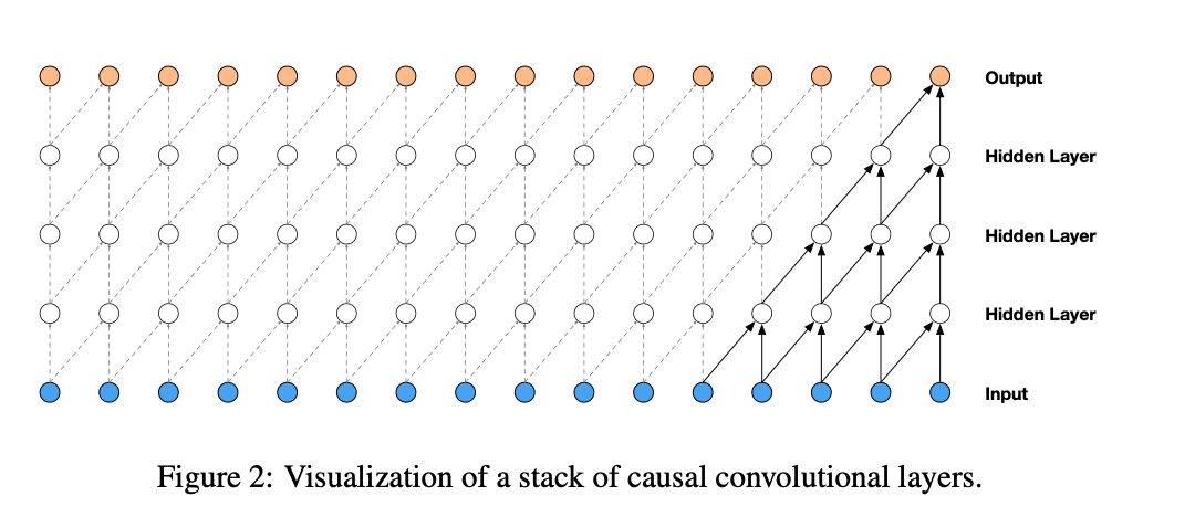
This is like an experienced trader who not only watches the micro博弈 on the 5-minute line but also occasionally switches to daily and weekly lines to observe macro trends.

Stacking causal convolution layers with different dilation rates forms the classic TCN (Temporal Convolutional Network). It cleverly achieves multi-cycle resonance in chart analysis using minimal computational resources.

Not a Guaranteed Win

Before treating causal convolution as a universal key, we must soberly recognize: it is still an inductive tool based on historical data.

If your raw data is essentially a random walk with extremely low signal-to-noise ratio and no discernible pattern, even if TCN opens up a large receptive field, what it extracts will just be a concentration of noise.

It cannot conjure Alpha out of thin air.

But undeniably, it provides us with an extremely handy tool. It can safely (without look-ahead bias) compress a period of price-volume trends into a feature vector.

Whether this vector is input into a fully connected layer for return prediction, or used as the environment state (State) in reinforcement learning algorithms, it demonstrates high engineering value and computational efficiency.

This article is part of our Factor Analysis and Machine Learning Strategies series, specifically in the section on handling time-series features. The important results obtained from causal convolution will serve as the core features for training our deep learning strategies. We will discuss more on how to驾驭 these models in our class!

💡 Final Note: When applying TCN in live trading, the biggest pitfall is often not in the network structure, but in data preprocessing. Feeding absolute prices that have not been processed for stationarity or cross-sectional standardization directly into the network will likely cause the model to become confused.

As Jim Simons, founder of Renaissance Technologies, said: "In this business it's easy to confuse luck with brains." When you make money using advanced causal convolution, don’t assume the model has some magical power; it might just be fitting the current market sentiment. In quantitative finance, we must always remain in awe of the market’s chaos.