TCN for Quant: Clearer Time-Series Deconstruction

Many friends new to quantitative deep learning have a first reaction: run LSTM or GRU.

I was the same when writing my thesis. At the time, I thought Recurrent Neural Networks (RNNs) were tailor-made for financial sequences: they have "memory" and can handle temporal logic.

I eagerly fed years of price-volume data from China A-shares into an LSTM, fantasizing about generating a perfect prediction curve.

Reality slapped me hard.

No matter how I tuned the parameters or added layers, the LSTM’s predictions always seemed to be "chasing the rally and selling the crash"—it was essentially just shifting yesterday’s prices. When market conditions changed abruptly, the model collapsed.

My advisor then said, "Why not try TCN (Temporal Convolutional Network)?"

To be honest, I was resistant at first. Aren’t Convolutional Neural Networks (CNNs) for image recognition?

Using them for K-line charts felt like a misuse of technology. Plus, when I tried it, TCN’s performance on that paper’s data was merely passable, lacking that "dimensional strike" magic.

But as I kept hitting walls, I realized TCN’s true value isn’t in boosting accuracy by a few points, but in reconstructing time series with extremely clear, extremely "quantitative" logic.

In quantitative modeling, we are essentially solving one problem: how to allocate weights to historical data.

In our previous article, we discussed how causal convolutions replace MA/EMA, letting the model learn weights itself: $$ y_t = \sum_{i=0}^{k-1} w_i \cdot x_{t-i} $$

If causal convolutions solve "how to allocate weights to history," then TCN (Temporal Convolutional Network) solves "how to build a multi-scale feature pyramid."

But if you’ve already accepted causal convolutions, a question soon arises: since the convolution kernel can already learn weights, why do we need TCN?

Because causal convolutions only solve "how to allocate weights to recent history," they don’t solve "how to safely incorporate more distant history."

Assume the kernel size $k=3$. It can only look at 3 time steps at a time. This is fine for short-term fluctuations; but if you want to simultaneously judge intraday noise, weekly momentum, and monthly trends, a 3-step view is clearly too narrow. You could violently stack the network deeper, but as layers increase, training becomes unstable.

So, TCN’s first step isn’t inventing a new network, but doing "seeing further" more cleanly on top of causal convolutions.

In our previous article, we covered Dilated Convolution. It transforms the standard causal convolution $$ y_t = \sum_{i=0}^{k-1} w_i \cdot x_{t-i} $$

into $$ y_t = \sum_{i=0}^{k-1} w_i \cdot x_{t-d\cdot i} $$

Sampling along the time axis with stride $d$.

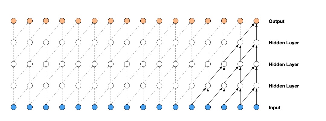
When $d=1$, it’s identical to standard causal convolution; when $d=2, 4, 8$ expand layer by layer, the receptive field expands exponentially. If we view each layer as a convolution operation, a common result is: $$ RF = 1 + (k-1)(2^L - 1) $$

This means you don’t need to stack the network to an exaggerated depth to bring days, weeks, or even months of history into view.

In common residual block implementations in TCN papers, each block typically串s two dilated convolutions, so the actual receptive field is often even larger than this formula suggests.

This is where TCN’s true value lies: it doesn’t simply stretch history; it processes information at different time scales within the same convolutional framework.

Each layer of TCN processes information at different scales:

• Bottom layers ($d=1, 2$): Capturing high-frequency volatility and order-book jumps (short-term micro-trading).
• Middle layers ($d=4, 8$): Extracting weekly momentum or mean reversion (medium-term博弈).
• Top layers ($d=16, 32$): Examining multi-month trends or seasonality (long-term格局).

By stacking multi-layer dilated convolutions, TCN maintains sensitivity to minute-level fluctuations at the bottom while capturing weekly or even monthly trends at the top.

This "exponentially expanding" view allows TCN to cover ultra-long historical spans with very shallow layers, avoiding the gradient vanishing problem common in deep recurrent networks like LSTM.

Depth Robustness: How to Keep Deep Networks "Alive" in Noise?

With dilated convolutions, we can "see" far, but the accompanying question is: the network gets deeper.

In image processing, deep networks are king; in quantitative finance, deep networks are often a disaster.

Financial data has a very low signal-to-noise ratio and severe non-stationarity. Simply stacking convolutional layers causes the model to quickly lose its way in gradient vanishing or explosion, or fall into the swamp of overfitting.

TCN’s true essence lies in finding an excellent balance between "depth" and "robustness" through a Residual Block structure.

Residual Blocks: From "Predicting Price" to "Predicting Deviation"

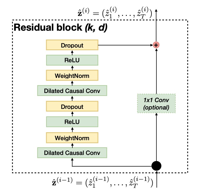
So, TCN’s second step is adding a constraint to deep networks: "don’t mess things up." This is the residual block. It writes each layer’s output as: $$ \mathbf{y} = \sigma(\mathbf{x} + \mathcal{F}(\mathbf{x})) $$

Where $\mathbf{x}$ is the raw input, and $\mathcal{F}(\mathbf{x})$ is the correction learned by the convolutional layer.

Many articles introducing ResNet say the residual block’s role is to "alleviate gradient vanishing." That’s correct, but it’s too light for time-series modeling.

More accurately, the residual block changes the problem itself. Originally, the network learned a complete mapping $H(\mathbf{x})$; now it learns only: $$ \mathcal{F}(\mathbf{x}) = H(\mathbf{x}) - \mathbf{x} $$

The deviation from the raw input.

This rewrite is particularly important in quantitative finance. Price sequences have strong autocorrelation; predicting the next moment, the current price is the most natural benchmark.

The residual structure tells the model: you don’t need to reconstruct the entire price curve from scratch every time; you only need to answer a more realistic question—is there a deviation worth correcting on the current benchmark?

From an optimization perspective, this structure has a harder benefit. During backpropagation, the gradient’s derivative with respect to input becomes: $$ \frac{\partial \mathbf{y}}{\partial \mathbf{x}} = I + \frac{\partial \mathcal{F}}{\partial \mathbf{x}} $$

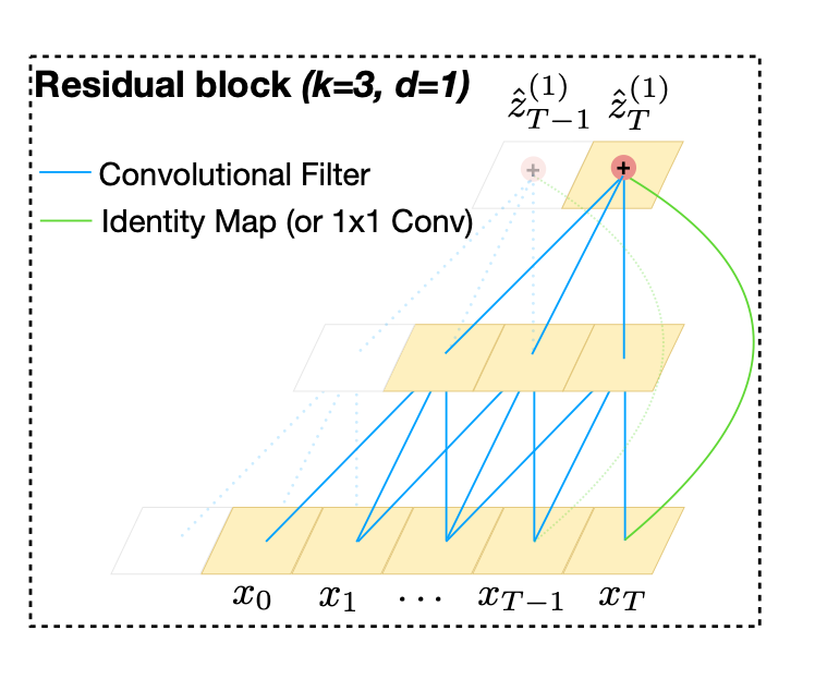
The $I$ in that identity mapping is critical. It means that even if the convolutional branch initially learns nothing, the gradient still has a nearly direct path back.

For deep TCN, this is more important than "learning a few more features," because financial sequences fear not insufficient model complexity, but the network twisting the most original, stable price structure when it gets deep.

If a layer extracts no effective Alpha, the best approach isn’t to force a complex transformation, but to let $\mathcal{F}(\mathbf{x})$ stay close to 0, passing the signal through unchanged.

Precisely because of this, the residual block leaves space for "self-degeneration" in deep TCN: if it can’t learn Alpha, at least it won’t destroy the original price structure.

But residuals aren’t enough. To stabilize deep network training, we must also solve the optimization path itself.

Many tutorials casually add Batch Norm, but it’s not popular in time-series tasks. Batch Norm standardizes activation values as: $$ \hat{x} = \frac{x - \mu_B}{\sqrt{\sigma_B^2 + \epsilon}} $$

Where $\mu_B$ and $\sigma_B^2$ come from statistics within a batch.

This is usually fine for images, as images default to sharing statistical structures; but in financial time series, it’s dangerous.

Today’s volatile market, tomorrow’s one-way market, and next week’s sudden negative news are simply not the same distribution.

Rubbing these time slices into a single batch to calculate mean and variance is essentially forcing the assumption that they share the same "normal state." What you often get isn’t more stable features, but features averaged out and flattened, erasing regime differences.

TCN more commonly uses Weight Normalization. It doesn’t touch activation values but directly reparameterizes weights: $$ \mathbf{w} = g \frac{\mathbf{v}}{|\mathbf{v}|} $$

Separating weight magnitude and direction. The benefit isn’t prettier code, but more stable optimization.

During gradient updates, there’s no need to entangle "which direction to go" and "how big a step to take," making deep networks easier to converge. Crucially, it doesn’t mix statistical quantities from different time slices, making it more suitable for sequences where distributions drift at any time.

Finally, Dropout. Many treat it as a catch-all for "preventing overfitting," but in TCN, it serves a specific engineering role. During training, it applies a Bernoulli mask to features: $$ \tilde{\mathbf{h}} = \mathbf{m} \odot \mathbf{h}, \quad m_i \sim \text{Bernoulli}(1-p) $$

Meaning that during each forward pass, some pathways are temporarily cut off.

This is particularly important in financial modeling: because financial data contains too much accidental noise, if a layer happens to capture a price-volume combination valid only in-sample, the network easily mistakes it for a true rule.

Dropout forces the model not to rely on a single path, but to seek structures that repeat across different samples.

You can also view it as a very crude model ensemble: training occurs on different sub-networks each time, and what remains stable at the end is often not the flashiest signal, but the one least prone to distortion.

Simply put, TCN isn’t just "a bit more advanced" than causal convolutions. It builds on causal convolutions to fix two more problems: how to incorporate more distant history, and how to avoid corrupting signals when the network gets deeper.

12345678910111213141516171819202122class TemporalResidualBlock(nn.Module):
    def __init__(self, in_ch, out_ch, k, d, dropout=0.2):
        super().__init__()
        self.conv1 = CausalConv1D(in_ch, out_ch, k, d)
        self.conv1.conv = nn.utils.weight_norm(self.conv1.conv)
        self.relu1 = nn.ReLU()
        self.drop1 = nn.Dropout(dropout)
        
        self.conv2 = CausalConv1D(out_ch, out_ch, k, d)
        self.conv2.conv = nn.utils.weight_norm(self.conv2.conv)
        self.relu2 = nn.ReLU()
        self.drop2 = nn.Dropout(dropout)
        
        self.res = nn.Conv1d(in_ch, out_ch, 1) if in_ch != out_ch else nn.Identity()

    def forward(self, x):
        out = self.relu1(self.conv1(x))
        out = self.drop1(out)
        out = self.relu2(self.conv2(out))
        out = self.drop2(out)
        
        return nn.ReLU()(out + self.res(x))

Looking back, what truly impresses me about TCN isn’t that it’s newer than LSTM, nor that it wins a few points on a specific dataset, but that it clearly dissects several of the most troublesome problems in time-series modeling:

First,守住 causality; second, expand the view; finally, ensure depth doesn’t destroy the raw signal.

This is why I increasingly treat it as a feature extraction framework rather than a panacea for prediction.

It can’t conjure Alpha out of thin air, but it at least provides a clean, stable way to help us organize chaotic historical sequences into something worth further research.