
CSI 1000 Bottom-Fishing: 95% Win Rate on Sharp Drawdowns
On April 8, we published an article titled "1-to-10 Odds: I Bottomed the Market on March 27," using robust statistical evidence to justify why that specific date was optimal for entering long positions. Six months later, the CSI 1000 has provided two new examples. This article reviews those findings.
Principles and Definitions
Let’s first outline the underlying logic. You may have observed that during consecutive down trends, the deeper the decline, the stronger the subsequent rebound, and the higher the probability of a reversal. It’s like a spring or bungee jumping: after falling continuously to a certain point, the price always snaps back somewhat.
However, we need to determine precisely how deep the consecutive decline must be to calculate the probability of a rebound. This gives our trading strategy a solid foundation and rationale.
First, we must define "consecutive decline." As mentioned in previous articles, we could use daily price changes. However, in this article, we attempt a different approach: defining the decline based on the drop within consecutive bearish candle intervals. This filters out many false signals.
The specific calculation method is shown below:
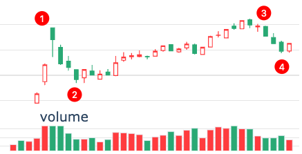
Let’s look at the segment from point 1 to point 2 in the figure. This represents the price action from October 8 to October 11. On October 8, the market gapped up but then fell continuously until October 11. For buyers entering at the open on the 8th, the loss at the close on the 11th reached 15.8%. This loss is what we define as the drop within a consecutive bearish candle interval.
Now, consider the segment from point 3 to point 4. This covers November 14 to November 18. Buyers entering at the open on the 14th incurred a loss of 7.5%; thus, the drop within the consecutive bearish candle interval is 7.5%.
If we calculated the maximum drop using consecutive daily declines (rather than consecutive bearish candle intervals), we would start counting from November 12. However, this would trigger a bottom-fishing signal prematurely on November 15. This signal would be too early because a "fake bullish candle" occurred on November 13 (price fell but closed higher). On this day, chips changed hands. Assuming those who lost money the previous day sold all their positions to new entrants, the holding cost for active traders decreased, allowing them to withstand further pressure for a while.
This is why we improved the definition to use the drop within consecutive bearish candle intervals. In practice, both definitions have pros and cons; you can use a machine learning model to decide which definition to apply in different market conditions.
Code Implementation
With the model definition clear, let’s implement it. This code requires a function to detect consecutive bullish/bearish candles, which we define as find_runs:
def find_runs(x):
"""Find runs of consecutive items in an array.
"""
# ensure array
x = np.asanyarray(x)
if x.ndim != 1:
raise ValueError("only 1D array supported")
n = x.shape[0]
# handle empty array
if n == 0:
return np.array([]), np.array([]), np.array([])
else:
# find run starts
loc_run_start = np.empty(n, dtype=bool)
loc_run_start[0] = True
np.not_equal(x[:-1], x[1:], out=loc_run_start[1:])
run_starts = np.nonzero(loc_run_start)[0]
# find run values
run_values = x[loc_run_start]
# find run lengths
run_lengths = np.diff(np.append(run_starts, n))
return run_values, run_starts, run_lengthsTo ensure reproducibility, we use akshare to provide data. This is a free, open-source market data source.
import akshare as ak
now = datetime.datetime.now().date()
start = now - datetime.timedelta(days=365*4)
start_date = start.strftime("%Y%m%d")
end_date = now.strftime("%Y%m%d")
# Fetch CSI 1000 daily data (last ~1000 days) via akshare
bars = ak.index_zh_a_hist(symbol="000852", start_date=start_date, end_date=end_date)
bars.rename(columns = {
"日期": "date",
"开盘": "open",
"最高": "high",
"最低": "low",
"收盘": "close",
"成交量":"volume"
}, inplace=True)
bars["date"] = pd.to_datetime(bars["date"])
bars.set_index("date", inplace=True)
bars["flag"] = np.select([bars["close"] > bars["open"],
bars["close"] < bars["open"]],
[1, -1],
0)
v, s, l = find_runs(bars["flag"] == -1)
cum_neg_returns = []
for vi, si, li in zip(v, s, l):
if vi and li > 1:
cum_neg_returns.append((bars.index[si],
bars.index[si + li-1],
bars.close[si + li -1 ]/bars.open[si] - 1))
r = pd.DataFrame(cum_neg_returns, columns=["start", "end", "cnr"])
r.cnr.hist()Looking at the generated histogram, occurrences where the consecutive drop exceeds 7.5% are rare. In other words, it is a low-probability event for the price to continue falling after a consecutive decline of more than 7.5%.
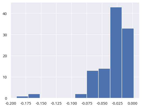
Let’s examine the 10 most severe consecutive declines:
r.nsmallest(10, "cnr").sort_values("end", ascending=False)| start | end | cnr | |
|---|---|---|---|
| 107 | 2024-11-14 | 2024-11-18 | -0.075433 |
| 106 | 2024-10-08 | 2024-10-11 | -0.158511 |
| 89 | 2024-03-21 | 2024-03-27 | -0.071948 |
| 88 | 2024-01-26 | 2024-02-05 | -0.190592 |
| 87 | 2024-01-19 | 2024-01-22 | -0.067846 |
| 78 | 2023-10-16 | 2023-10-23 | -0.074109 |
| 45 | 2022-09-15 | 2022-09-19 | -0.066983 |
| 37 | 2022-04-20 | 2022-04-26 | -0.170335 |
| 34 | 2022-03-14 | 2022-03-15 | -0.066983 |
| 33 | 2022-03-03 | 2022-03-09 | -0.086669 |
We see five such events in 2024: January 22, February 5, March 27, October 11, and most recently, November 18. The declines on February 5 and October 11 were particularly severe, leading to significant rebounds. Indeed, the bigger the storm, the bigger the fish!
The inclusion of the January 22 event in this table is surprising, as the decline lasted only two days. However, it did trigger a small rebound lasting three days with gains exceeding 6.1%, which is quite substantial.
How to Bottom-Fish?
At the close on November 8, the consecutive bearish candle drop was 7.54%, with intraday drops being even larger. Thus, during the trading day, a consecutive drop of 7.54% occurred. If you decided to bottom-fish at that moment, what is the probability of success?
A somewhat quirky pandas function helps us calculate this:
decline_ratio = -0.075433
r.cnr.le(decline_ratio).mean()The cleverness lies in using le (less than or equal) to identify data points less than or equal to decline_ratio, marking them as True and others as False. Applying mean to these boolean variables calculates the proportion of True values, which is exactly the probability we seek!
This probability is 4.63%. If you bottom-fish at this point, there is a 4.63% chance you will need to endure further declines, as happened on October 9. Following the probabilistic hint, you would likely enter the market on the afternoon of October 9 and endure two more days of decline, with a drop similar to what you previously observed (around 7.5%).
However, the good news is that if you entered on October 9, you have the option to exit with a small profit on October 10. If you exit on that day, selling your chips to new entrants, they can withstand another 7.5% drop! This explains the stock market proverb: "As long as bulls survive, the decline continues."
If you are not a programmer, you can use the following table to quickly check the success rate of bottom-fishing:
data = []
for loss in np.linspace(-0.06, -0.076, 15):
data.append((loss, 1- r.cnr.le(loss).mean()))
df = pd.DataFrame(data, columns=['最大亏损', '抄底胜率'])
df.style.format("{:.1%}")| 最大亏损 | 抄底胜率 | |
|---|---|---|
| 0 | -6.0% | 87.0% |
| 1 | -6.1% | 87.0% |
| 2 | -6.2% | 87.0% |
| 3 | -6.3% | 87.0% |
| 4 | -6.5% | 88.0% |
| 5 | -6.6% | 89.8% |
| 6 | -6.7% | 90.7% |
| 7 | -6.8% | 93.5% |
| 8 | -6.9% | 93.5% |
 Follow us on WeChat: Quantide Daily quant insights, strategy research and tool tutorials. |