Rescuing CCI: Factor Purification Reveals a Powerful Technical Signal

The Commodity Channel Index (CCI), developed by Donald Lambert and first published in the Commodity Futures magazine in 1980, has long been highly regarded by traders. However, using this indicator directly as a factor for factor testing nearly obscured its value. Ultimately, the factor density distribution revealed the truth: through factor purification, the final testing results aligned with traditional experience.

The CCI calculation formula is:

$$ CCI=\frac{Typical Price - MA}{.015 * Mean Deviation} $$

Where,

$$ \text{Typical Price}t=(H_t+L_t+C_t)\div 3 \ MA = Moving Average \ Moving Average = (\sum{i=1}^PTypical Price)\div P \ Mean Deviation = (\sum_{i=1}^P|Typical Price - MA|)\div P $$

In simple terms, CCI represents the deviation of price from the moving average.

The idea behind CCI—using the average of the **highest price, lowest price, and closing price as the price series**—is common in many contexts. Essentially, **it is an approximation of VWAP**. Therefore, if VWAP data is available, using it directly might be better, as its market meaning is clearer.

There is a "magic number" in the CCI formula: 0.15. Its purpose is to standardize the CCI value to a reasonable range, giving signal significance at the boundaries of -100 and 100. Initially, the formula’s designer, Lambert, believed that when CCI is within the [-100, 100] range, prices are fluctuating randomly and are not worth trading. Only when the absolute value of CCI exceeds 100 is a trend considered to have emerged—i.e., buy when CCI crosses above 100, and sell when it crosses below -100.

Let’s first observe this indicator using a simple dual-axis chart.

123456789df = PAYH.copy()
df['cci'] = ta.CCI(df.high, df.low, df.close, 14)

axes = df[['close', 'cci']].plot(figsize=(14, 7), 
                            subplots=True, 
                            title=['PAYH', 'cci'])
axes[1].set_xlabel('')
sns.despine()
plt.tight_layout()

Here is the output:

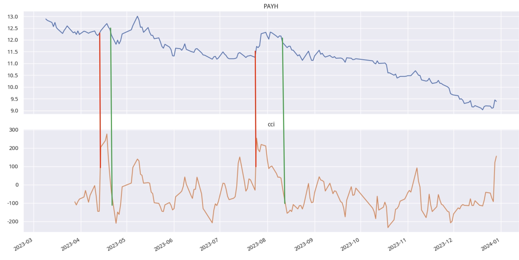
In the output, I marked trading signals at two points where CCI crossed $\pm 100$ to illustrate its signaling role. This is merely an observation of a single asset over a short period and does not prove much on its own.

Now, let’s run factor testing to evaluate it:

12345_ = alphatest(2000, start, end, 
              calc_factor = lambda x: ta.CCI(x.high, 
                                             x.low, 
                                             x.close, 
                                             14))

The factor testing results appear poor.

However, a slight analysis of CCI’s principle makes it clear that it is not suitable for use as a direct factor. This is because CCI’s trading signal is triggered when CCI crosses $\pm 100$. It is an event signal, not a factor in the conventional sense.

Let’s explain why from the perspective of factor distribution.

1234567891011cci = barss.groupby(level="asset")
            .apply(lambda x: ta.CCI(x.high, 
                                    x.low, 
                                    x.close, 
                                    timeperiod=14
                                    )
                )

with sns.axes_style('white'):
    sns.distplot(cci)
    sns.despine()

Looking at the density distribution, the factor distribution is bimodal.

As we discussed in the course, if a factor’s distribution is bimodal, it often contains multiple influences and is not pure. We are currently facing this situation. In such cases, for factor analysis, we must first "purify" the factor.

12345678cci = barss.groupby(level="asset")
            .apply(lambda x: ta.CCI(x.high, 
                                    x.low, 
                                    x.close, 
                                    timeperiod=14))
with sns.axes_style('white'):
    sns.distplot(cci[cci> 0])
    sns.despine()

The output results are as follows:

Now, the distribution of CCI is unimodal. Let’s proceed with factor testing to see the results:

12345678910def calc_cci(df, n):
    cci = ta.CCI(df.high, df.low, df.close, n)
    cci[cci < 0] = np.nan
    return cci * -1
    
alphatest(2000, 
         start, 
         end, 
         calc_factor= calc_cci, args=(14,), 
         max_loss=0.55, long_short=False)

Note that in the third line of this code, we corrected the returned CCI by setting negative values to NaN, so they will be discarded during factor testing. This was covered when we discussed the Alphalens framework.

Because we discarded half of the factors, when calling Alphalens, we need to set the max_loss parameter to be greater than 0.5 (refer to the maxlosserror report for details).

Based on the purified factor, the returns are impressive. It is not as strong as the RSI we tuned previously, but since we are in a pure long position scenario, the results are particularly attractive.

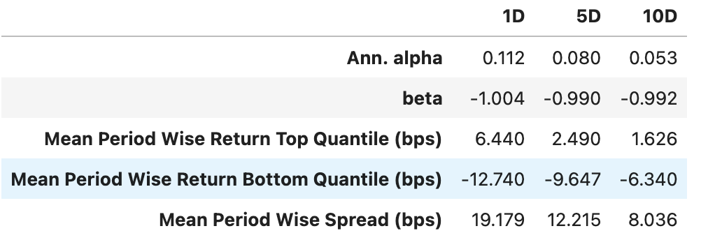
Alpha reached 19% annually. Moreover, this factor exhibits good positive monotonicity, as seen in the layered backtest returns:

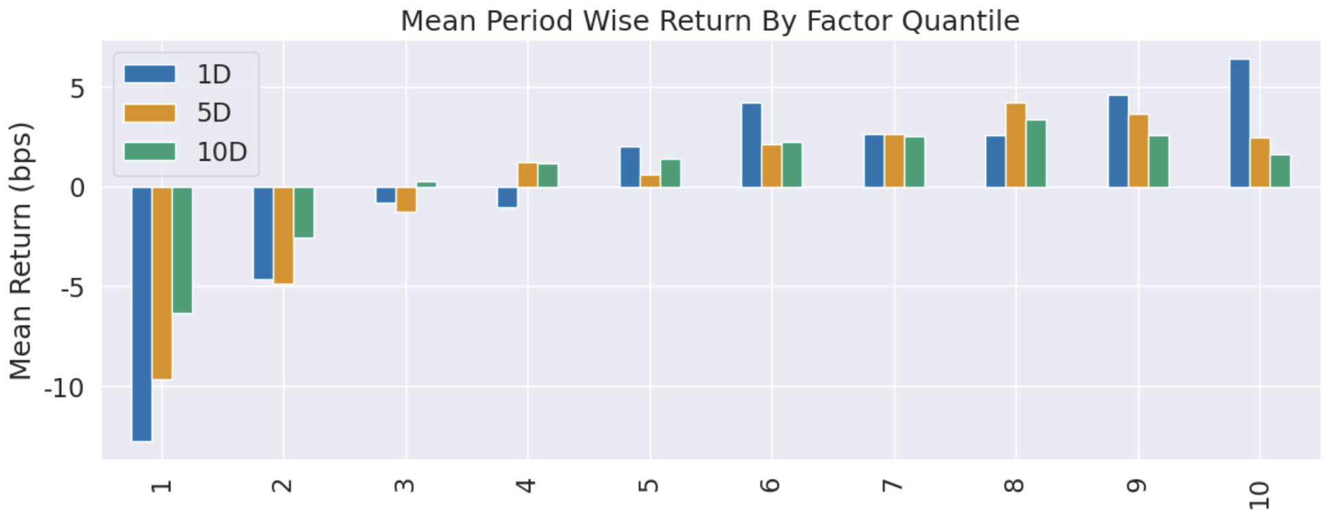
However, its cumulative return performance in a pure long position is not very stable. This is also evident from the beta value in the annual return chart above, showing significant sensitivity to market volatility.

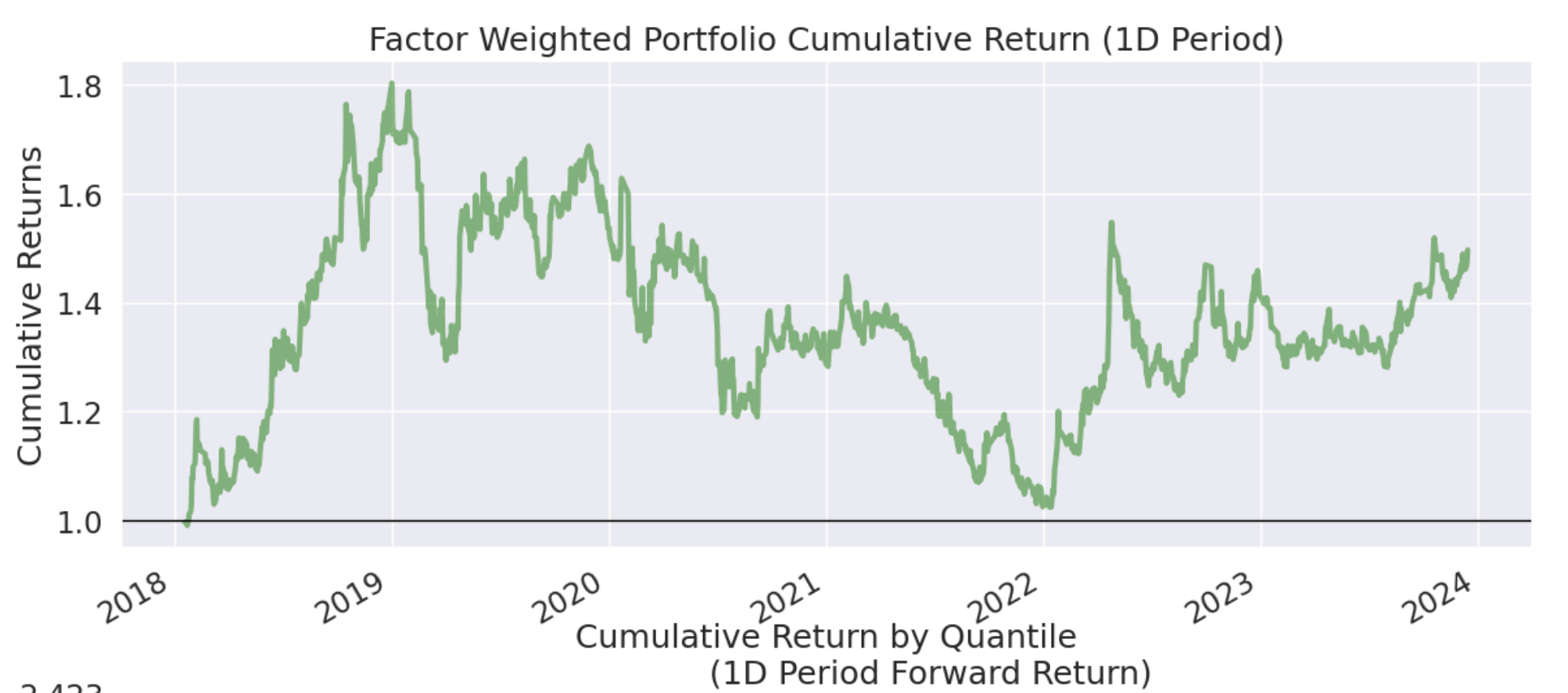
But we don’t necessarily have to stick to a pure long position; CCI was originally a futures indicator. Let’s look at the long-short portfolio scenario:

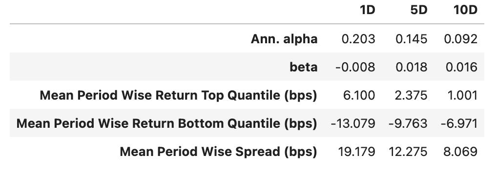
Not only is the Alpha return strong, but the beta is hedged to nearly zero! With beta at zero, the cumulative return should be steadily upward with low volatility. Let’s see if this holds true:

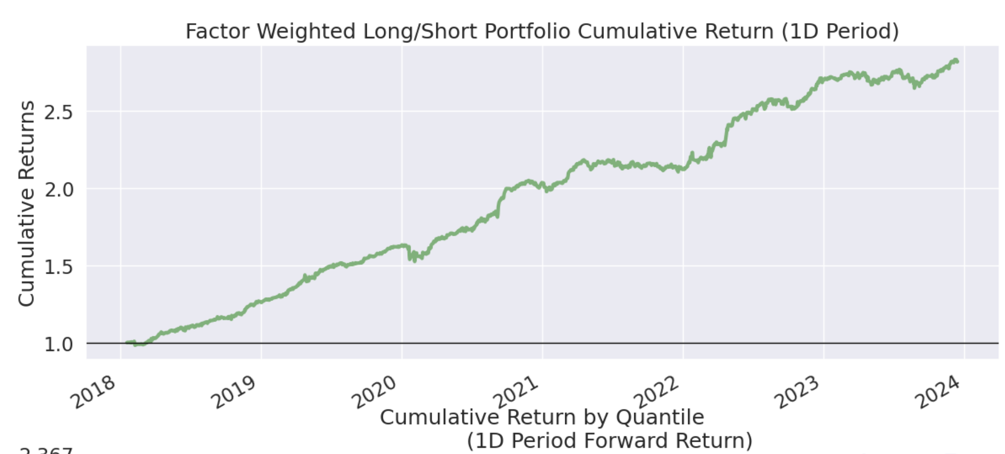
This may be one reason why CCI is so highly regarded.

However, this factor testing is not equivalent to live trading, as the operational methods differ. In factor testing, we execute weighted long-short operations based on factor values. In live trading, positions are opened or closed based on fixed conditions of whether CCI crosses $\pm 100$. In factor testing, our entry conditions are looser, offering some adaptive characteristics.

This article includes code and data for reproducibility. Join the community to access the Jupyter Notebook research environment and run the code directly.

In this environment, in addition to the code from this article, the code from previous paid articles is also available. Furthermore, any future articles that declare the inclusion of reproducible code and data can be found in this environment.