CSI 1000 Bottom-Fishing: How a 10-to-1 Payoff Emerges

In my March 28 article, I explained why the previous day's sell-off was foreseeable. In this follow-up, I use hard statistics to show why that was the day to buy the dip, and what the expected risk-reward looked like.

Buying the dip isn't about greed. It's about getting ahead early to lower risk. In the darkest hour, remember: there is no final success, no fatal failure — what counts most is the courage to keep going!

---

Calculating Odds and Expected Return

On March 27, the Shanghai Composite fell 1.26% while the CSI 1000 dropped 3.33%, with losses widespread. In Lesson 14, we asked: when the Shanghai Composite drops 4%, what is the probability that buying the dip succeeds? Using that question, we introduced PDF/CDF concepts and showed how to solve it with ECDF in statsmodels and related methods in numpy/scipy.

But in practice, a more relevant question is when China A-shares have fallen x% in a row, what is the expected profit-loss ratio — the so-called odds — if you buy the dip here? On March 27 this year, we got a live example: the CSI 1000 closed down 6.943% cumulatively, then rebounded 5.5% in a row — a very sizable gain.

We have already covered everything needed to solve this in earlier lessons. The most important tool is find_runs, introduced in Lesson 9.

It splits an array into groups of identical consecutive values, returning each group's value, start position, and length.

With it, we can locate the endpoints of every consecutive down-run from daily returns and compute the pnl for each run:

12returns = bars.close.pct_change()
v, s, l = find_runs(returns <= 0)

The returns array holds daily returns. Through the returns <= 0 expression, we get a binary array where True means the market did not rise that day — it fell or closed flat.

We get the following result:

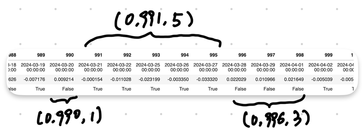
The result is an array of triplets, each in the form (v, s, l), representing the current group's value, start position, and length.

Next, we loop over this array, use s and l to find each run's start and end, and compute the run's gain/loss from the closing prices at the two endpoints. Below we only compute the down-runs:

12345678close = bars.close
cum_neg_returns = []
for vi, si, li in zip(v, s, l):
    if vi and li > 1:
        cum_neg_returns.append((bars.frame[si-1], bars.frame[si + li - 1], close[si + li - 1]/close[si-1] - 1))
        
r = pd.DataFrame(cum_neg_returns, columns=["start", "end", "cnr"])
r

This gives us 116 results:

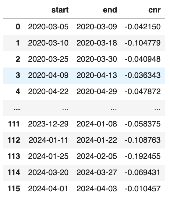
At the March 27 close, we were at row 114 of the table above — the CSI 1000 had fallen continuously from March 20 to March 27, for a cumulative drop of 6.94%.

So what was the probability of further decline? It is equivalent to (s < x).sum()/len(s), but let's use a different approach:

12p_decline = r.cnr.le(-0.06943).mean()
p_decline

The output is 0.0862. In other words, over the past four years there were 116 episodes of consecutive declines lasting 2 days or more. Of those 116, when the closing drawdown reached 6.943%, the probability of further decline was 8.62% — implying a 91.38% chance of a rebound.

If it doesn't rebound, we suffer a loss on our dip purchase. What is the expected loss? Let's look at the cases that kept falling after -6.94%:

1r[r.cnv < -0.0694]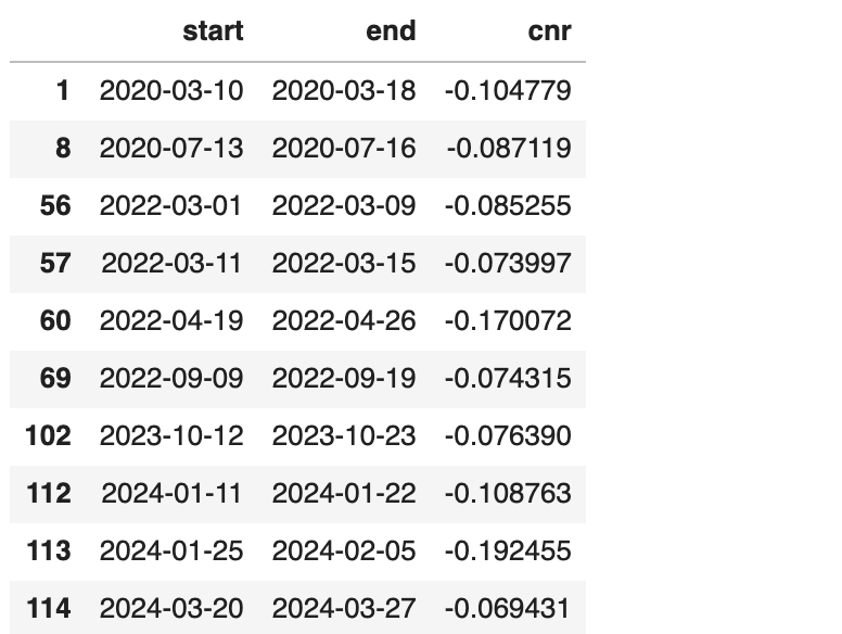

Its expectation is:

1234# 抄底失败的亏损预期

exp_lose = (r[r.cnr<-0.06943].mean() - (-0.0694))
exp_lose

A failed dip-buy — i.e., continued decline — occurred 10 times, with an average loss of around -10%. Since we only bought after -6.94%, our incremental loss would be about 3.48%. Remember, the probability of this happening was only 8.62%.

If it rebounds, how much would we make? This is slightly trickier to compute. After March 27, the rebound reached 5.5%. But that is just a single sample — we can't assume every rebound will be that large.

Let's take a conservative approach: treat all rebounds following declines in the [-5%, -6.943%] range as proxies for rebounds after -6.943%. Clearly, in a sharp sell-off, the deeper the drop, the stronger the bounce, so this will underestimate the rebound after -6.94%. But it also gives our model an extra margin of safety.

12345678910# 抄底时间为bounced
bounced = [f.date() for f in (r[(r.cnr >= -0.0695) & (r.cnr<-0.05)]["end"])]

# 抄底收益为bounced之后，连接上涨的收益

cum_pos_returns = []
for vi, si, li in zip(v, s, l):
    end = tf.day_shift(bars.frame[si], -1)
    if end in bounced:
        cum_pos_returns.append((bars.frame[si-1], bars.frame[si + li - 1], close[si + li - 1]/close[si-1] - 1))

12profit = pd.DataFrame(cum_pos_returns, columns=["start", "end", "profit"])
profit

The code above first identifies rebound dates, then loops over the triplets we obtained earlier. If the day before a run's start was the end of a consecutive down-run, we compute that run's gain. The resulting expected gain is:

1234# 抄底的收益期望是

exp_win = profit.profit.mean()
exp_win

This expectation is 3.299%. That looks similar to the expected loss if the dip-buy fails, but to compute the odds we must weight by probabilities:

$$ exp_win * 91.38% / (exp_lose * 8.62%) = 10.03% $$

Finally, the overall expected value of buying the dip is:

$$ exp_win * 91.38% + exp_lose * 8.62% = 2.71% $$

With DMA and 4x leverage, a single trade would gain more than 10%.

Rougher Seas, Bigger Fish?

Years ago, my partner recommended Nassim Taleb's The Black Swan. Honestly, the first quarter of the book is brilliant, but the rest felt hard to put into practice.

Aside: I actually prefer Natalie Portman's film Black Swan.

Still, I have never stopped thinking about black-swan events. From a different angle, treating black swans as low-probability events to be studied quantitatively seems worthwhile. It breaks from the book's framework, but at least it gives us a starting point.

But some may ask: why try to catch a falling knife? Isn't it better to make money steadily? The problem is, this market rarely offers steady-money opportunities.

If you don't secure first-mover advantage at the lows with cheap chips, you easily end up trapped halfway up the mountain or at the peak. In fact, if you didn't enter on March 27, the recent rally was very hard to capture.

Buy the dip! Based on solid statistical odds, getting ahead early to stay invincible is the only way to survive in this market.

A Bonus Surprise

In our calculation, a failed dip-buy was provisioned at the maximum loss. But in practice, in a sharp sell-off, the harder the fall, the stronger the rebound — readers can verify this themselves.

Here is the point: we provisioned about 3% average loss for a failed dip-buy. But we didn't account for what happens after being trapped by 3%. Take the harshest rout this year, from January 25 to February 5: if we had bought the dip at -6.94%, would we really have lost 3%?

You can verify it yourself. In fact, that round fell fast and bounced hard. If we had bought after a 6% drop, we would have bought the CSI 1000 at around 4984, suffered about a 13% drawdown, but ultimately ridden consecutive rebounds to 4993 — ending with a 0.18% gain.