A-Share Valuation: PE Percentiles vs. The Low-PE Trap

A heart-stopping scene unfolded before the holidays, with major indices hitting their lowest weekly closes of the year. Naturally, we want to understand the current market state: are there undervaluation opportunities? In this article, we examine whether these conditions present genuine opportunities or potential traps through the lens of price-to-earnings (PE) ratios.

We use akshare to retrieve the Shanghai Composite Index PE data. Note that this data originates from the LeguLegu website.

1234567import akshare as ak

pe = ak.stock_market_pe_lg(symbol="上证")
pe.set_index("日期", inplace=True)
pe.index.name = "date"
pe.rename(columns={"平均市盈率": "pe", "指数": "price"}, inplace=True)
pe.tail(15)

This yields all data since 1999, formatted as follows:

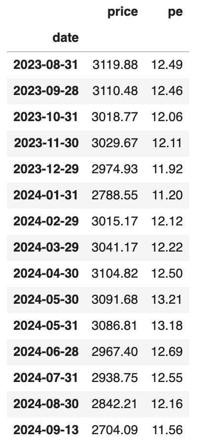
Undervalued in August?

We can use the quantile function to identify the 25th, 50th, and 75th percentiles of the PE distribution:

12345percentiles = []
for i in range(1, 4):
    percentiles.append(pe["pe"].quantile(i/4))

percentiles

Since 1999, the 25th, 50th, and 75th percentiles have been 13.9, 17.4, and 33.5, respectively.

So, where does the Shanghai Composite Index’s PE stand as of late August 2024?

We can calculate this position using the following method:

123rank = pe.rank().loc[datetime.date(2024,8,30), "pe"]
percentile = rank / len(pe)
percentile

The results show that the current PE is at approximately the 10.6th percentile, placing it in a relatively low position since 1999.

Based strictly on statistical percentiles, it appears the Shanghai Composite Index was undervalued at the end of August 2024, implying a buying opportunity.

However, percentiles are static and do not reflect the trend of the data.

PE Trends

If you open the Eastmoney client and view the Shanghai Composite Index’s profile page, you can see its historical PE trend. The chart over the past decade is as follows:

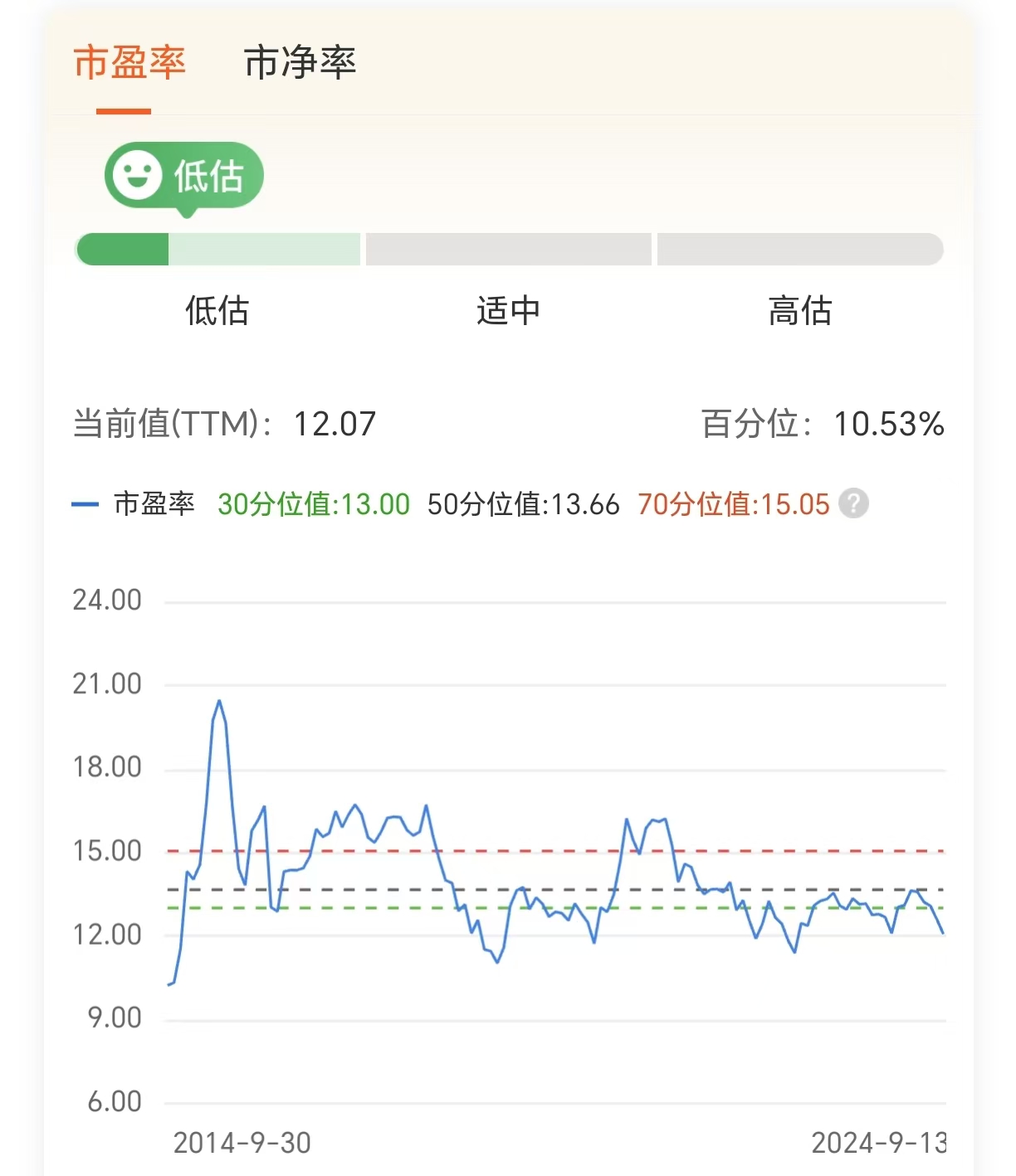
This chart, however, does not provide additional insight. From this view, the Shanghai Composite Index still appears undervalued.

Let us overlay the historical price trends onto the PE trends to see if PE peaks and troughs truly correspond to price peaks and troughs.

123456789101112131415161718192021222324252627282930import matplotlib.pyplot as plt
import matplotlib.dates as mdates

fig, ax1 = plt.subplots(figsize=(60,6))

color = "tab:blue"
ax1.plot(pe["price"], label="Index", color=color)
ax1.set_xlabel("Year")
ax1.set_ylabel("Index", color="tab:blue")
ax1.xaxis.set_major_locator(mdates.MonthLocator(bymonth=[2, 5, 8, 11]))
ax1.xaxis.set_major_formatter(mdates.DateFormatter('%Y-%m')) 

color = "tab:red"
ax2 = ax1.twinx()
ax2.plot(pe["pe"], label="PE", color=color)
ax2.set_ylabel("PE", color=color)

for i in range(1, 4):
    quantile = pe["pe"].quantile(i/4)
    ax2.axhline(quantile, color='gray', linestyle='--', label=f"{i/4:02.0%}")

plt.title("Index vs PE")

fig.tight_layout()
for date in pe.index[::3]:
    ax1.axvline(date, color='gray', linestyle=':', linewidth=0.5)
plt.gcf().autofmt_xdate()

plt.legend(loc="upper left")
plt.show()

This generates the following plot:

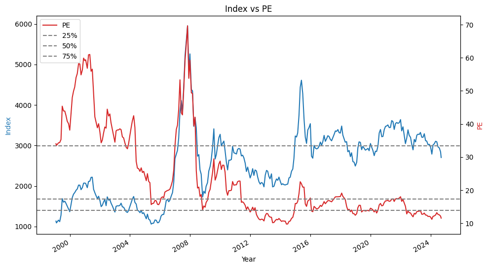
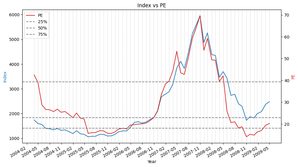
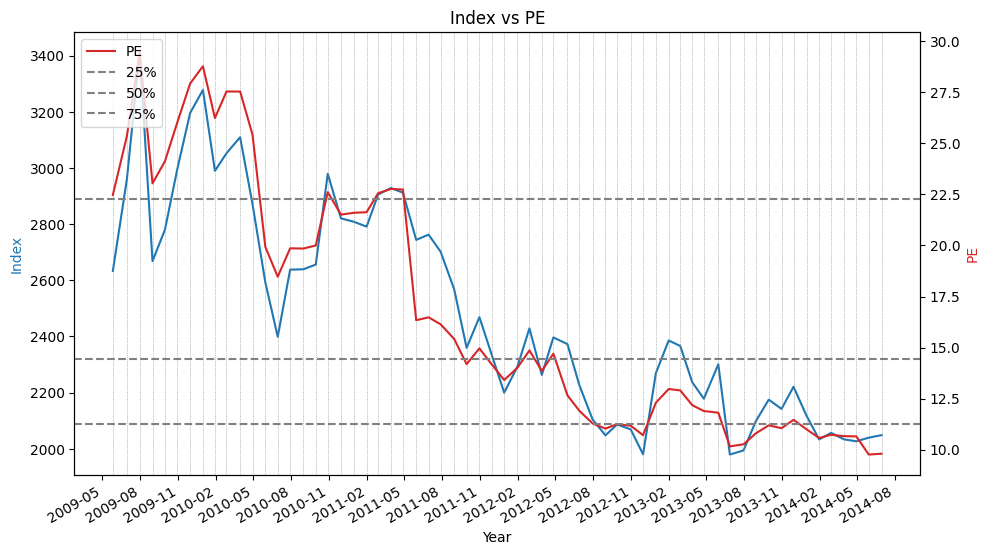
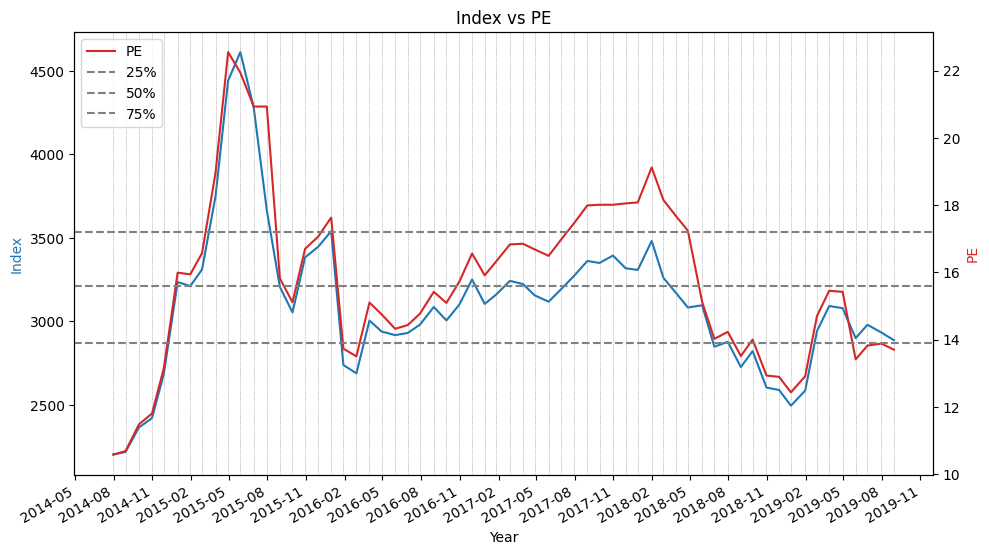
The chart reveals that from 1999 to 2024, there has been a general trend of rising Shanghai Composite Index prices accompanied by declining PE ratios. The index’s rise likely reflects the long-term trend of GDP growth, while the decline in PE is primarily due to the expansion of asset supply, which continuously squeezes out asset bubbles.

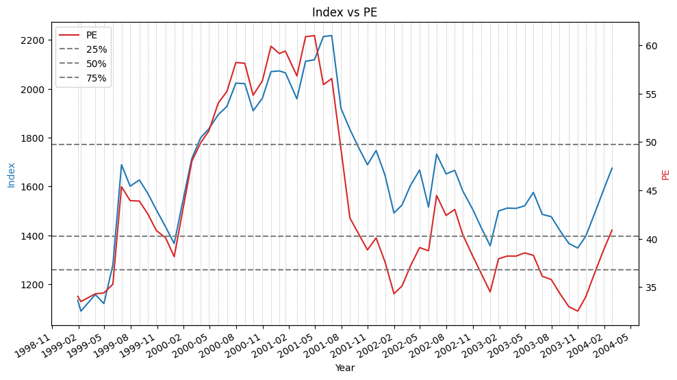
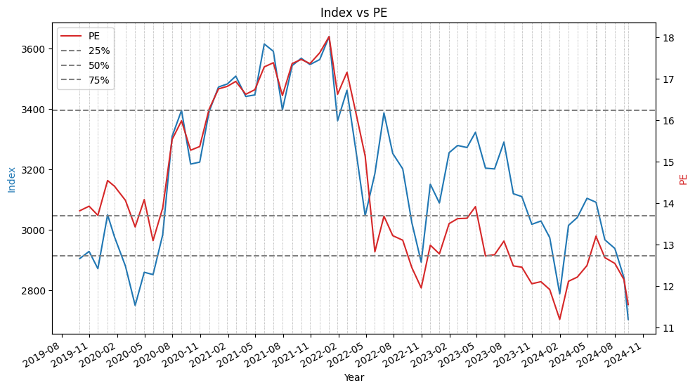
To examine these details more closely, we have split the above chart into five subplots:

Reflections and Conclusions

• Question: During which periods did the PE trend move in perfect lockstep with the Shanghai Composite Index? In such movements, which is the dependent variable and which is the independent variable? What phenomenon does this reflect?

• Answer: Between 1999–2001, August 2005–May 2008, and May 2014–May 2015, the PE trend moved in perfect lockstep with the Shanghai Composite Index. During these periods, market speculation was intense, and changes in corporate earnings were negligible relative to price changes. Consequently, the PE trend was entirely driven by stock prices, causing the PE curve to closely mirror the price trend. When this phenomenon occurs, it indicates that the market has become excessively speculative.

• Question: Since approximately August 2023, it appears that the Shanghai Composite Index has declined faster than PE. For instance, in February 2024, both the index and PE hit阶段性 lows. However, in September 2024, while the index hit a new low, PE did not. What phenomenon does this divergence reflect? Can it be described using a common term?

• Answer: In September 2024, after the Shanghai Composite Index hit a new low, PE did not follow suit, creating a divergence. This can also be observed through peak analysis. For example, in June 2024 (see Table 1), PE reached a new high since August 2023, while the index remained below any high point since August 2023. This divergence can be described as the low-PE trap. This indicator reminds us that while the index is falling, the profitability of listed companies may also be declining, leading to scenarios where the index rises slightly while PE surges, or the index falls significantly while PE declines only modestly.

Therefore, if we rely solely on percentile statistics, current A-shares appear undervalued. However, considering the overall downward trend in PE and the recent divergence between PE and index movements over the past year, determining whether A-shares are truly undervalued remains questionable. A more multidimensional assessment is required.

This article is derived from the exercises in Lesson 2 of Factor Analysis and Machine Learning Strategies.