Loss vs. Metrics: Why MAPE Fails as XGBoost Objective

Today we'll look at how MAPE is used in the paper. We'll use it as an opportunity to go a bit deeper into machine learning fundamentals and cover two topics:

Loss Functions vs. Metrics

In machine learning, there are two important classes of functions: objective functions, also known as loss functions, and metrics.

The loss function drives training. During training, methods like gradient descent keep pushing the loss lower until it cannot go any lower — at which point training is done.

Once training is finished, the model is tested on a test set, and its predictions are compared against ground truth. To quantify that comparison, we introduce metrics.

sklearn provides a large collection of loss functions and metrics. The figure below shows a subset of what sklearn offers:

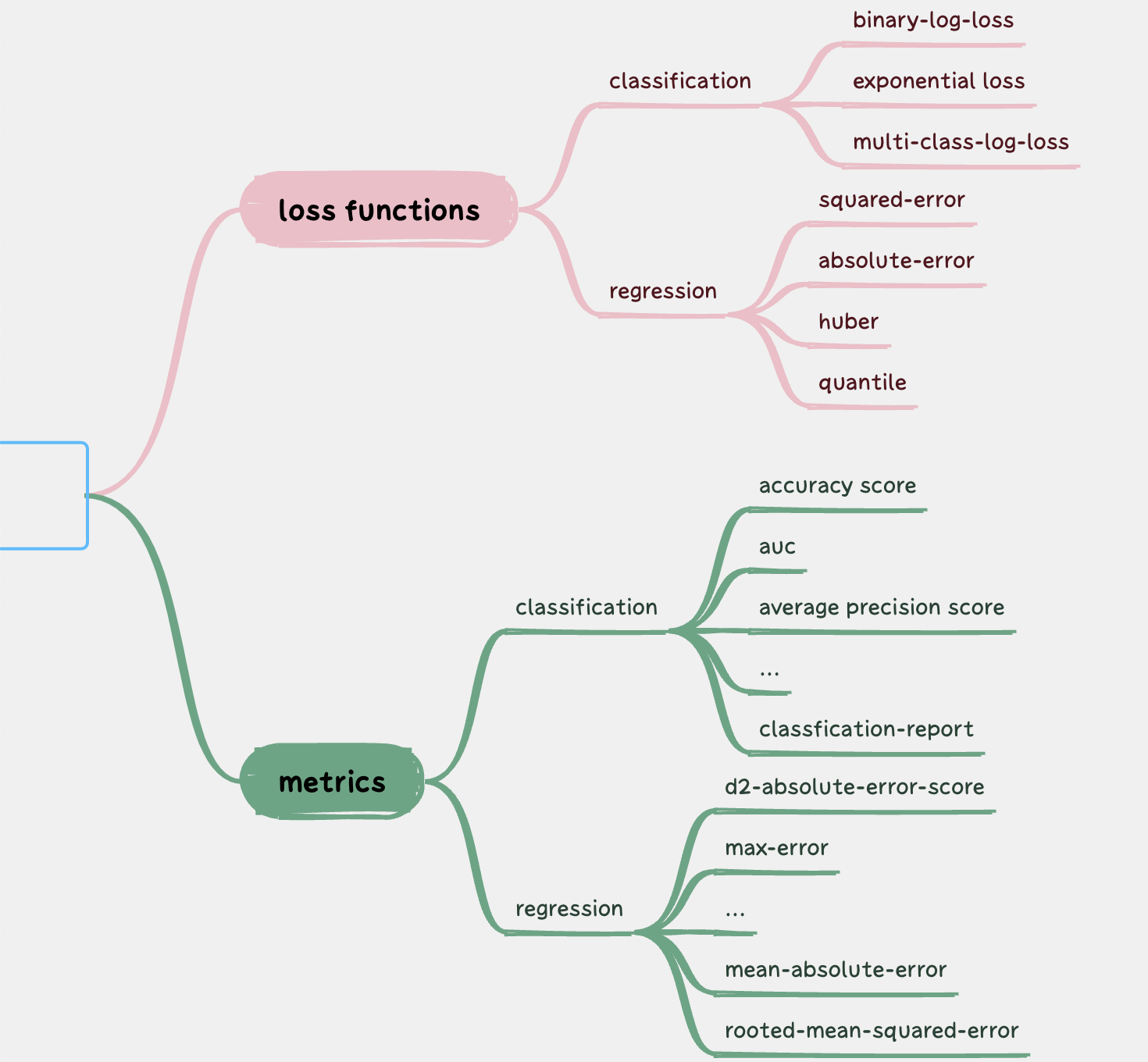
Notice that there are far more metrics than loss functions. Why?

In the paper, the author does not disclose the actual XGBoost training procedure, only saying that the XGBoost database was used directly. That phrasing is odd — we can read it as using XGBoost defaults. But he specifically highlights MAPE, which from the workflow is clearly used as a post-hoc evaluation metric.

In XGBoost, if no objective is specified, the default is RMSE (root mean square error) with a regularization penalty. RMSE can also serve as a metric. In the paper, the author does not use RMSE as the metric, but instead chooses MAPE (mean absolute percentage error). Why? And if MAPE is better in this setting, why not train with MAPE?

At first glance, both objectives and metrics want predictions to be as close to actuals as possible. If they share that property, why distinguish between them?

To answer that, you need to understand how XGBoost is trained — specifically, how it does gradient descent.

XGBoost: Second-Order Taylor Expansion

XGBoost is a boosting algorithm. It stacks many weak learners to form a strong learner. At each iteration, the new tree corrects the residual of the existing model — that is, the difference between predictions and actuals. The size of that difference is measured by the objective function.

In XGBoost, the stacking of weak learners uses an additive model: the final prediction is the weighted sum of all weak-learner outputs. This structure lets us approximate the loss function with a Taylor expansion for efficient optimization.

XGBoost optimizes the objective via a second-order Taylor expansion and then solves using second derivatives. With second-order information, XGBoost converges much faster, because it considers not only the direction of the gradient but also the shape of the loss function.

$$ f(x) \approx f(a) + f'(a)(x-a) + \frac{f''(a)}{2!}(x-a)^2 $$

It is this internal optimization mechanism that dictates our choice of objective: the objective must be twice differentiable.

RMSE is twice differentiable, but MAPE is not: by definition MAPE can be zero, and around those zero points even the first derivative does not exist, let alone the second. Here is the MAPE formula:

$$

\text{MAPE} = 100\frac{1}{n}\sum_{i=1}^{n}\left|\frac{\text{实际值} - \text{预测值}}{\text{实际值}} \right| $$

When the prediction matches the actual value, MAPE is zero.

How to Choose an Objective?

Choosing MAPE as the metric is not just about making different models comparable — in finance it has special significance:

We care far more about relative error between prediction and truth than absolute error. In trading, percentage is king. For that reason, if we could train with MAPE as the objective, the resulting accuracy would be much closer to real-world use than accuracy obtained by training with RMSE.

This is an entry point for improving algorithms in a specific domain. A loss function called SMAPE has already been proposed for this purpose:

$$

\text{SMAPE} = \frac{100}{n} \sum_{t=1}^n \frac{\left|F_t-A_t\right|}{(|A_t|+|F_t|)/2} $$

So far sklearn does not provide this function, but we can implement it ourselves and plug it into sklearn via make_scorer:

123456789101112from sklearn.metrics import make_scorer

def smape(y_true, y_pred):
    return np.mean(2.0 * np.abs(y_pred - y_true) / 
           (np.abs(y_true) + np.abs(y_pred)))

smape_scorer = make_scorer(smape, greater_is_better=False)

# 使用举例：在GridSearchCV中使用
grid_search = GridSearchCV(estimator=model, 
                           param_grid=params, 
                           scoring=smape_scorer)

Question: If MAPE cannot be used in training, why does the paper use MAPE in testing?

The answer is actually simple: to make multiple models comparable. In the author's setup, every stock gets its own model. Since each stock trades at a very different absolute price, their RMSE values are not comparable, while MAPE is effectively a normalized measure. It therefore allows comparison across models so the stocks with the smallest error can be selected for the strategy universe.

But as noted before, the author's model is not meaningful — a classification model would be better. And if you switch to classification, the loss is no longer RMSE, and the metric can no longer be MAPE.

Standardization

The paper also mentions that factor data were standardized before training.

In fact, that step is pointless. Because XGBoost is a tree model: it splits and partitions data by comparing feature values. Those split comparisons do not depend on units or scale, so standardization serves no purpose and may even cause precision loss — more harm than good.

Also, the paper trains one model per stock. But what if you used a single model and trained it 1,000 times on data from 1,000 stocks? Then you clearly must standardize up front. Otherwise convergence will be very difficult — although even with standardization, convergence is not guaranteed. Whether it converges depends on whether all those stocks truly share the same feature-to-label mapping. That is not a requirement of XGBoost itself, but an extra requirement imposed by how we choose to use XGBoost.

Conclusion

For most quants, building a machine learning framework from scratch like Chen Tianqi did is out of reach. So to get better results from the same model, the only levers are data labeling, objective functions, evaluation functions, and hyperparameter tuning. That usually demands both deep domain knowledge and a solid understanding of how the model actually works.

Finally, my new book Efficient Python Programming: A Practical Guide (《Python高效编程实践指南》, China Machine Press) is now available. If you are a quant looking to level up your engineering skills, it is an ideal choice. Self-recommendation here.