Is an 85% Accurate ML Model a Money Printer?

In Lesson 13, after introducing the principles of machine learning via decision trees, some students began actively considering whether they could integrate the various factors they had previously studied—typically used in single-factor models—into a single strategy using a decision tree model.

After discussing with students, I’ve shared this approach. This is also the exercise for Lesson 13, and I’m sharing the reference answer here.

Preview: The model we trained achieves an astonishing F1-score of around 85% across all three classes on both the validation and test sets!

How is this model constructed?

Feature Data

First, we select the features. We chose the following factors, all of which were introduced in the course and for which source code is provided:

1. First-derivative factor: Reflects the trend of an individual stock over a period.
2. Second-derivative factor: Predicts short-term trend reversals effectively.
3. RSI factor: A classic technical factor that can predict tops and bottoms to some extent.
4. Weekday factor: Adds a new dimension completely unrelated to the aforementioned price-volume information.

The implementation of these factors is as follows:

12345678910111213141516171819def d2_factor(df, win: int = 2)->pd.Series:
    close = df.close/df.close[0]
    d1 = close.diff()
    d2 = d1.diff()
    factor = d2.rolling(win).mean()
    
    return factor

def rsi_factor(df, win: int = 6)->pd.Series:
    return ta.RSI(df.close, win)


def d1_factor(df, win: int = 20)->pd.Series:
    df["log"] = np.log(df.close)
    df["diff"] = df["log"].diff()
    return df["diff"].rolling(win).mean() * -1

def week_day(dt: pd.DatetimeIndex)->pd.Series:
    return dt.weekday

The training data spans six years, from 2018 to the end of 2023, with 2,000 individual stocks randomly sampled as the universe.

12345start = datetime.date(2023, 1, 1)
end = datetime.date(2023, 12, 29)

np.random.seed(78)
barss = load_bars(start, end, 2000)

The first three factors above are time-series factors. However, when we mined these factors, we used Alphalens, which performs layered ranking. Therefore, we must also rank these factors cross-sectionally to generate rank_* factors. This approach is equivalent to feature augmentation.

12345678910111213141516171819202122features = {
}

def rank_feature(feature):
    return feature.groupby(level=0).rank(pct=True)

for name, func in [("d2", d2_factor),
                   ("rsi", rsi_factor),
                   ("d1", d1_factor)]:
    feature = barss.groupby(level=1).apply(d2_factor).droplevel(0)
    features[name] = feature
    features[f"rank_{name}"] = rank_feature(feature)

# Calculate rank
features = pd.DataFrame(features)
features['weekday'] = week_day(features.index.get_level_values(0))

for win in (1, 5, 10):
    features[f"ret_{win}"] = barss.groupby(level=1)["price"].pct_change(win)
    
features.dropna(how='any', inplace=True)
features.tail()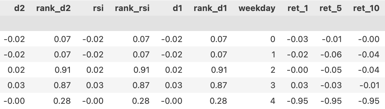

The output is the feature dataset.

The columns ret_1, ret_5, and ret_10 represent the returns for the next 1, 5, and 10 days, respectively. Following our previous practice, returns are calculated based on the rule: buy at the opening price of T1 and sell at the opening price of T2, for each time point T0. When training the model, only one column is used at a time.

Regression or Classification?

Now, we face the choice of how to transform the above data into trainable data. There are three questions:

1. How to select the model? Even if we decide to use a decision tree, we must still choose between regression and classification.
2. How to split the training and test sets? This appears to be the simplest step among all questions.
3. Can we use data from different samples simultaneously as training inputs? This question seems somewhat complex.

Given our selected features, having the model perform regression tasks seems unreasonable; classification makes more sense, but requires some transformation. We recommend using a classification model and splitting the test set using sklearn’s built-in train_test_split.

1234567from sklearn.model_selection import train_test_split

X = features.filter(regex='^(?!ret_).*$')
y = np.select((features["ret_1"] > 0.01, 
               features["ret_1"] < -0.01), 
              (1, 2), default=0)
X_train, X_test, y_train, y_test = train_test_split(X, y, test_size=0.2, random_state=42)

We label returns greater than 1% as class 1, returns less than -1% as class 2, and the rest as class 0. Label 0 can also be considered as "unclassifiable."

We train the model using the following code:

123456789101112from sklearn.tree import DecisionTreeClassifier
from sklearn.metrics import accuracy_score, classification_report

# Initialize and train the model
clf = DecisionTreeClassifier(random_state=42)
clf.fit(X_train, y_train)

# Predict and evaluate the model
y_pred = clf.predict(X_test)

print("Accuracy:", accuracy_score(y_test, y_pred))
print("Classification Report:\n", classification_report(y_test, y_pred))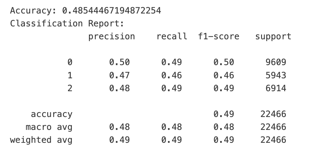

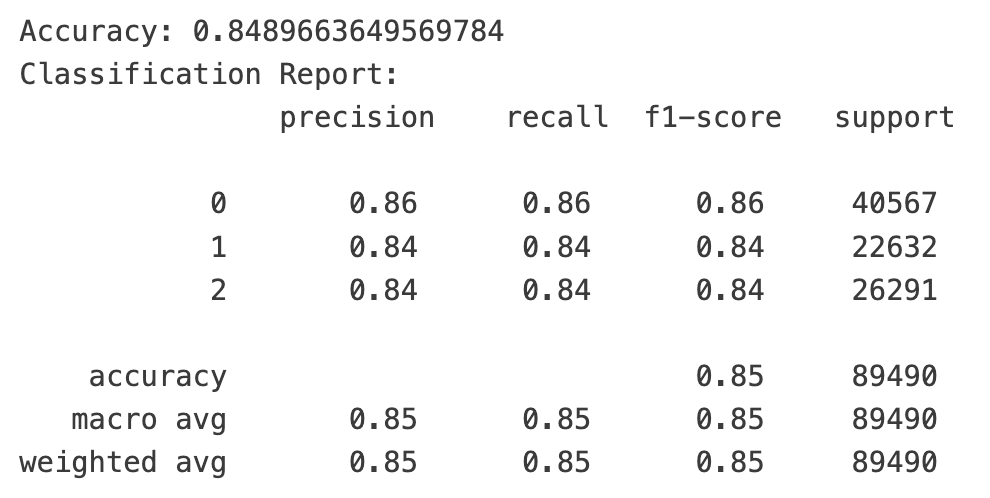
The results are extremely satisfying. In a three-class problem, random guessing yields an accuracy of 33%. Our first run already far exceeds random guessing.

However, the support counts for the three classes are not balanced, which causes some concern: Will the dominance of class 0 lead to artificially high accuracy?

Rebalancing! Will the Report Look Bad After Undersampling?

Let’s address this issue first. We can use a method called undersampling, drawing samples from each class equal to the smallest sample count among the three. This way, the model sees relatively balanced training data.

Although implementing undersampling is simple, we have an even simpler method using the imbalanced-learn library:

123456789101112131415161718from imblearn.under_sampling import RandomUnderSampler

rus = RandomUnderSampler(random_state=42)
X_resampled, y_resampled = rus.fit_resample(X, y)

X_train_resampled, X_test_resampled, y_train_resampled, y_test_resampled = train_test_split(
    X_resampled, y_resampled, test_size=0.2, random_state=42
)

# Train the model
clf_resampled = DecisionTreeClassifier(random_state=42)
clf_resampled.fit(X_train_resampled, y_train_resampled)

# Predict and evaluate the model
y_pred_resampled = clf_resampled.predict(X_test_resampled)

print("Resampled Accuracy:", accuracy_score(y_test_resampled, y_pred_resampled))
print("Resampled Classification Report:\n", classification_report(y_test_resampled, y_pred_resampled))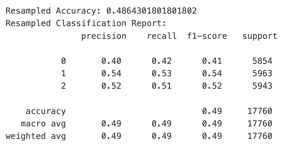

After class balancing, the overall accuracy remains largely unchanged, but the precision and recall for our classes of interest (class 1 and class 2) improved by 8% and 3%, respectively.

The results we just obtained are undoubtedly outstanding beyond expectations!

In the undersampled balanced version, if the model predicts that buying tomorrow will be profitable, its precision is 54%. That is, out of 100 predictions of profitability, 54 are correct; among the remaining 46 incorrect predictions, only 18 are losses, while the rest are fluctuations within 1%.

This analysis can be derived from the confusion matrix:

123456789from sklearn.metrics import confusion_matrix, ConfusionMatrixDisplay
import matplotlib.pyplot as plt

cm = confusion_matrix(y_test_resampled, y_pred_resampled)

disp = ConfusionMatrixDisplay(confusion_matrix=cm, display_labels=clf_resampled.classes_)
disp.plot(cmap=plt.cm.Blues)
plt.title('Confusion Matrix')
plt.show()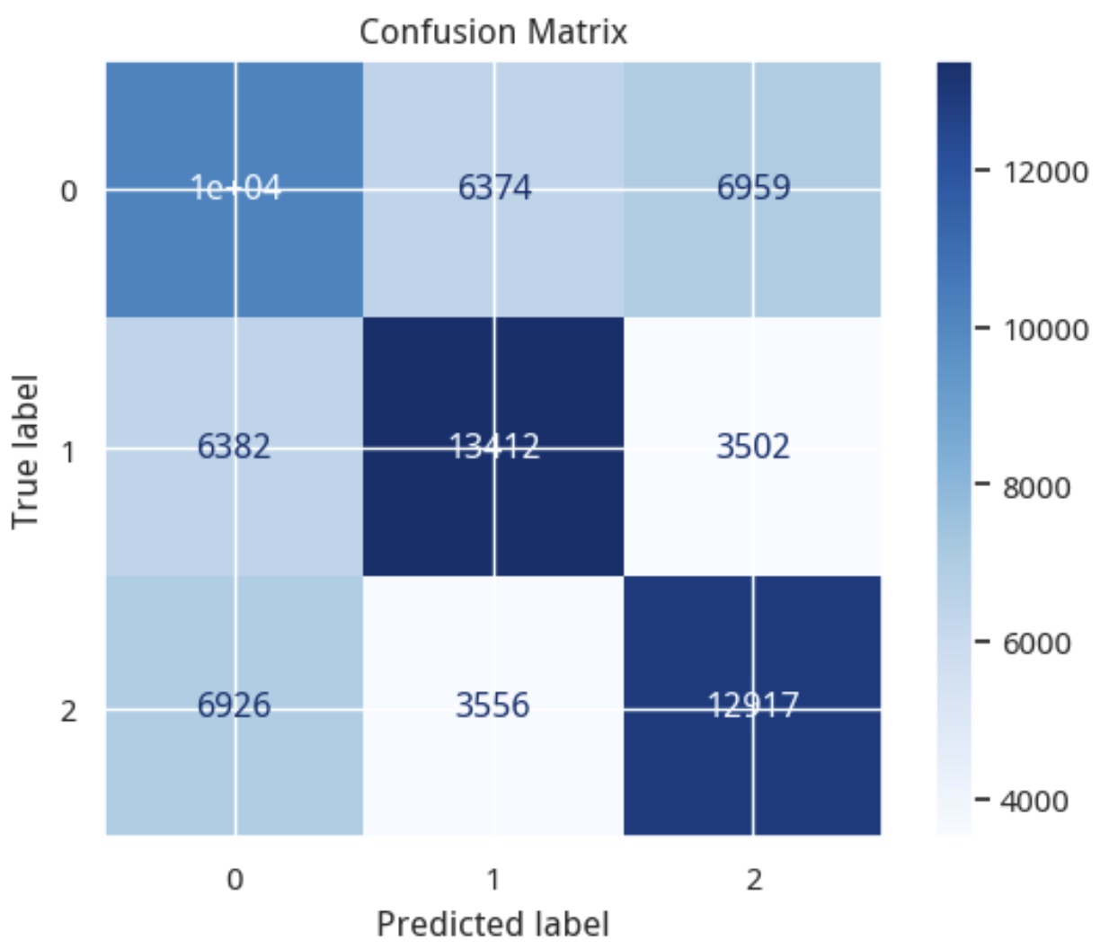

In the chart above, among samples predicted as class 1, 15% (3,556 samples) should actually be declining samples, and 27% (6,374 samples) are unknown (or flat) samples.

In reality, this represents a 57:15 profit-to-loss ratio, or a precision of 79%. How impressive is this? In Thorp’s gambling theory, he calculated that if the probability of winning exceeds 50%, one should bet. Because as long as the odds slightly favor oneself, through continuous accumulation, high-frequency trading can eventually accumulate considerable profits!

This might look very different from models you’ve seen elsewhere. You may never have imagined that machine learning models could be so effective in prediction. You might start looking for excuses, such as poor generalization or that the data only represents the past. But this is just the prelude; the climax is yet to come.

Although there are still areas for discussion in the construction of this model, it is indeed good enough because:

1. We provided high-quality feature data. We did not blindly pursue feature quantity. Thanks to our in-depth study in the first half of the Factor Analysis and Machine Learning Strategies course, we clearly understand which features can coexist harmoniously in a model, and we can even predict the contribution of each feature at specific nodes.
2. We know what results the features can produce, so we used the correct task model (classification) and employed certain construction techniques (gap handling).

Splitting training data into training and test sets is a very basic step in machine learning. Like many other tutorials, we used the train_test_split function here. It is simple and easy to use, but not suitable for quantitative trading.

It randomly samples training and test data, which tears apart the natural connections between data points and may even cause test set data to precede training set data, potentially leading to look-ahead bias.

The correct approach is to split by time order. sklearn provides a class called TimeSeriesSplit, which offers correct training and test set splits for cross-validation.

You can also use similar methods from the tsfresh library we introduced earlier to complete this task.

However, we don’t need cross-validation here, so we manually split the data into training, validation, and test sets.

X = features.filter(regex='^(?!ret_).*$') y = np.select((features["ret_1"] > 0.01, features["ret_1"] < -0.01), (1, 2), default=0)

n = len(X) X_train = X_train[:int(n0.7)] y_train = y_train[:int(n0.7)]

X_validation = X[int(n0.7):int(n0.9)] y_validation = y[int(n0.7):int(n0.9)]

X_test = X[int(n0.9):] y_test = y[int(n0.9):]

clf = DecisionTreeClassifier(random_state=42) clf.fit(X_train, y_train)

y_pred = clf.predict(X_validation)

from sklearn.metrics import accuracy_score, classification_report

print("Accuracy:", accuracy_score(y_validation, y_pred)) print("Classification Report:\n", classification_report(y_validation, y_pred))

123456
<!--027 6788 0230-->

<!-- BEGIN IPYNB STRIPOUT -->
![](https://cdn.jsdelivr.net/gh/zillionare/images@main/images/2024/12/decisiontree-made-easy-4.jpg)
<!-- END IPYNB STRIPOUT -->