
Translating Research into Code: 80% of the Work Explained
How to read and reproduce a research paper? This is a question frequently raised by our students.
Understanding and reproducing a research paper involves more than grasping the core idea. It requires mastering high-frequency industry terminology (jargon/slang), converting concepts into code, and knowing how to acquire data. These routine tasks account for 80% of the work. In our previous article on the RSRS Timing Indicator, we focused on reproducing the strategy itself. This article focuses on how to "translate" research papers.
In the research paper Market Timing Based on Relative Strength of Resistance and Support (RSRS) (hereinafter referred to as the "paper"), the key terms include: channel lines (Bollinger Bands), standard scores, linear regression, OLS linear regression, degrees of freedom, slope, total return, average annualized return, Sharpe ratio, max drawdown, net asset value (NAV), coefficient of determination, mean, standard deviation, skewness, kurtosis, correlation coefficient, and right-skewed standard scores. To read and reproduce this paper, you must understand these terms and concepts.
Many of these terms are standard statistical terminology, such as linear regression, slope, coefficient of determination, mean, and standard deviation. In Python, implementations for these can often be found in libraries like numpy, scipy, or statsmodels. However, we must note that different Python libraries, or even different versions of the same library, may implement these concepts with slight variations (which could be one reason why reproducing a paper fails).
For example, in numpy's linear regression, the order of returned alpha and beta differs between early and later versions. Similarly, the default values for degrees of freedom in covariance calculations may differ between numpy and scipy.

Other terms are common in the quantitative industry, particularly strategy metrics like Sharpe ratio and max drawdown. These are also implemented in well-known third-party libraries, which we will introduce later in this article.
Among these terms, we will focus on two concepts in this article: delta and standard scores.
Starting with Delta
Page 7 of the paper introduces the concept of $\Delta$ (delta), using the ratio $\Delta_{high}/\Delta_{low}$ to describe the relative strength of support and resistance levels, known as RSRS. This is the cornerstone of the entire paper, so we need to analyze it closely.
In mathematics, the symbol $\Delta$ generally represents a small change or increment. The limit of the ratio of two increments is the derivative, which geometrically corresponds to the slope. Therefore, the paper further explains:
Actually, delta (high) / delta (low) is the slope connecting two points on the high-low price plane: (low[0], high[0]) and (low[1], high[1]).
In quantitative scenarios, we sometimes see $\Delta_{close}$ (or $\Delta$ for other variables) referred to as a derivative. This is because the time increment of close is treated as 1, making the two numerically equivalent.

If we already understand these concepts, it becomes easy to understand the calculation rule for RSRS when $N=1$.
Then, considering that the slope between two points (i.e., RSRS with $N=1$) is too unstable, the paper proposes using linear regression over $N$ points to calculate the slope. In elementary mathematics, the slope is determined by the increments in the y-axis and x-axis directions of two points on a single straight line, i.e., $\frac{\Delta_y}{ \Delta_x}$.
If we view the slope as the angle of inclination, treating the line, X-axis, and Y-axis as vectors, the slope becomes the angle between two vectors. Since rotating both vectors simultaneously does not change their angle, we can calculate the slope via rotation. This extends the definition of slope from a single variable (fixing the other as the X-axis) to two variables.
In this generalized definition of slope, the slope reflects the proportion by which one variable changes when another variable changes. In quantitative finance, this indicates the magnitude of fluctuation in one linearly correlated variable when the other fluctuates. In this context, we refer to the slope as beta.
Based on the above discussion, it is now easy to understand that if we perform linear regression of variable Y on variable X, we obtain the beta of Y with respect to X, which is the slope.
$$ E(R_i) = R_f + \beta_i(E(R_m)-R_f) $$
The above equation is the CAPM formula proposed by William Sharpe. He was the first to use linear regression of individual stock returns against portfolio returns to derive the beta of individual stocks relative to the portfolio, later known as the market factor. Since then, linear regression between two variables has been widely applied in quantitative research. The method for calculating the RSRS indicator in the paper may have been inspired by this.
If we were to express the linear regression between two variables in code, it might look like this:
import numpy as np
X = np.arange(10)
y = X * 2 + np.random.randn(10)
(beta, alpha) = np.polyfit(X, y, 1)
print(beta, alpha)Of course, depending on user habits and data formats, you can also use corresponding methods in scipy and statsmodels.
Implementing Standard Scores in Code
Although "standard score" is a standardized term, if you transitioned from software or AI fields, you might be more familiar with its English name, Z-Score, rather than "standard score." This is something we must learn by reading more research papers and gaining practical experience.
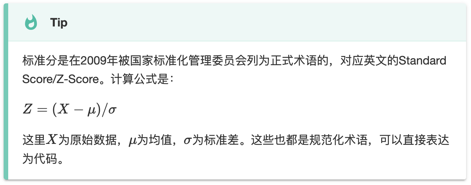
Once you understand that a standard score is a Z-score, it is easy to convert its formula into implementation code. In reproducing the research paper, we not only need to Z-score the raw RSRS factor but also implement Z-scoring under a sliding window efficiently. However, this implementation is simpler than calculating the slope under a sliding window, as it can be achieved using Pandas' rolling method and its broadcasting mechanism.
ZSCORE = (df["rsrs_"] - df["rsrs_"].rolling(m).mean())
/ df["rsrs_"].rolling(m).std()Pandas' rolling method returns an object that aligns well with multiple sliding window objects and supports broadcasting when operating with scalars. Therefore, this line of code reads like a mathematical formula.
These are skills that require practice and accumulation. In our article Factor Analysis and Machine Learning Strategies, we provided a detailed interpretation of the Alpha101 factors, including how to code various "operators." There, we introduced more techniques for coding operations mentioned in academic papers, including Z-score.
Coding Various Metrics
No strategy-related research paper can be separated from strategy evaluation.
There are many strategy evaluation metrics, and we generally do not need to implement them ourselves. However, we must understand the definition, calculation method, and key parameters of each metric. For example, annualized metrics often involve annualized multiples and the setting of risk-free rate parameters.
The starting point for calculating almost all strategy metrics is the periodic return. This can be a simple Python array, a Numpy array, or a Pandas Series. As long as we can calculate the strategy's periodic return (e.g., daily or monthly), the rest can be handed over to third-party libraries like empyrical and quantstats.
The former performs numerical calculations only, while the latter can also generate various reports, such as:
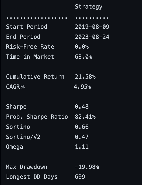
Therefore, before reading research papers, we can review the documentation and examples of these two libraries to understand how they implement numerical calculations and generate reports. Familiarity with these libraries will significantly accelerate the process of reproducing research papers.
Where Does the Data Come From?
This is indeed a question. It is not entirely a matter of technical capability; it also relates to costs.
To ensure that the reproduced research paper strategies and our public account articles can run, we have built a research platform (based on Jupyterlab). It provides daily data from 2005 to 2023 (cached). For other data, we can access it via the Tushare interface (using our shared Tushare premium account, valued at 500 RMB/year).