
Z-Transformed MA: Why a 12-Year-Old Strategy Still Beats the Market
Traditional Moving Averages (MA) are widely used trend-following indicators in technical analysis, calculated by averaging stock prices or indices over a specified number of days to depict directional changes. While a longer calculation window improves smoothness, it also exacerbates time lag (delay). This means MA indicators often struggle to "keep up" or even "follow" trends, creating an inherent trade-off between smoothness and latency.
The construction of the Low-Latency Trend (LLT) draws inspiration from filtering methods in signal processing theory. Traditional Exponential Moving Averages (EMA) act as first-order low-pass filters, but their filtering effect is relatively poor, with a transition band between the passband and stopband that is too wide. LLT optimizes this by designing a second-order filter, effectively filtering high-frequency signal components while preserving low-frequency intensity. Compared to traditional MA and EMA, LLT significantly reduces latency while maintaining trendline smoothness, thereby overcoming the lag issues inherent in traditional MA indicators.
This article is based on the Guangfa Securities report Low-Latency Trend Lines and Trading Timing. The original report backtested only until 2013. We extended the backtest to the end of 2024 and found that the strategy still performs well in long-short portfolios (Shanghai Composite Sharpe: 1.33).
Strategy Profile: LLT
| LLT | Benchmark | Strategy | | ----------------- | ---------- | ---------- | | Start Period | 2013-01-04 | 2013-01-04 | | End Period | 2024-12-31 | 2024-12-31 | | Cumulative Return | 47% | 345% | | CAGR﹪ | 2% | 9% | | Sharpe | 0.27 | 1.33 |For comparison, we first define and visualize traditional moving averages.
The Moving Average (MA) algorithm is:
$MA(n) = \frac{1}{n}\sum^{n-1}_{i=0}price(T-i)$
Here, price is typically the closing price, and $MA(n)$ represents the n-day MA indicator on day T. For MA indicators, a larger $n$ results in smoother trendlines.
Based on moving averages, we can implement a simple trend-following strategy. Signal generation is determined by the slope of the moving average line: if the slope is upward, maintain a long position; if downward, exit the long position.
The following code demonstrates 5, 10, 30, and 60-day moving averages. The 30-day MA is often referred to as the "lifeline." The final plot illustrates cases where the slope of the 30-day MA turns from positive to negative.
def get_price(symbol, start_date, end_date):
pro = pro_api()
price_df = pro.index_daily(
ts_code=symbol,
start_date=start_date.strftime("%Y%m%d"),
end_date=end_date.strftime("%Y%m%d"),
)
price_df = (
price_df.rename({"trade_date": "date", "ts_code": "asset"}, axis=1)
.sort_values("date", ascending=True)
.set_index("date")
)
return price_df[["close"]]
start = datetime.date(2012, 10, 26)
end = datetime.date(2013, 4, 9)
price_df = get_price("000001.SH", start, end)
for i in [5, 10, 30, 60]:
price_df[f"MA%d" % i] = price_df["close"].rolling(i).mean()
# Calculate lifeline trend inflection points
price_df["slope_30_5"] = price_df["MA30"].rolling(5, min_periods=5).apply(lambda y: np.polyfit(np.arange(5), y, 1)[0])
price_df["slope_30_5"] = price_df["slope_30_5"].fillna(0)
signs = np.sign(price_df["slope_30_5"])
sign_changes = signs * signs.shift(1) == -1
revert_dates = price_df.index[sign_changes]
print("Found reversal dates:", [i for i in revert_dates])
# Add tangents to the existing chart
cols = ["MA5", "MA10", "MA30", "MA60"]
ax = price_df[cols].plot(figsize=(18, 8), title='30-Day MA Tangent Analysis')
# Tangent length
tangent_length = 15
for dt in revert_dates:
# Get MA value and slope at this point
ma_value = price_df.loc[dt, 'MA30']
slope = price_df.loc[dt, 'slope_30_5']
i = price_df.index.get_loc(dt)
# Calculate tangent range
start_idx = max(0, i - tangent_length)
end_idx = min(len(price_df), i + tangent_length + 1)
# Calculate tangent coordinates
x_offset = np.arange(start_idx - i, end_idx - i)
y_tangent = ma_value + slope * x_offset
tangent_dates = np.arange(start_idx, end_idx)
# Draw tangent
color = 'green' if slope > 0 else 'red'
linestyle = '-.' if slope > 0 else '--'
ax.plot(tangent_dates, y_tangent,
color=color, linestyle=linestyle, linewidth=2, alpha=0.8)
# Mark tangent point
ax.scatter(i, ma_value, color=color, s=100, zorder=5)
ax.annotate(dt,
xy=(i, ma_value),
xytext=(5, 10), textcoords='offset points',
fontsize=9, color=color,
bbox=dict(boxstyle='round,pad=0.3', facecolor='white', alpha=0.8))
plt.show()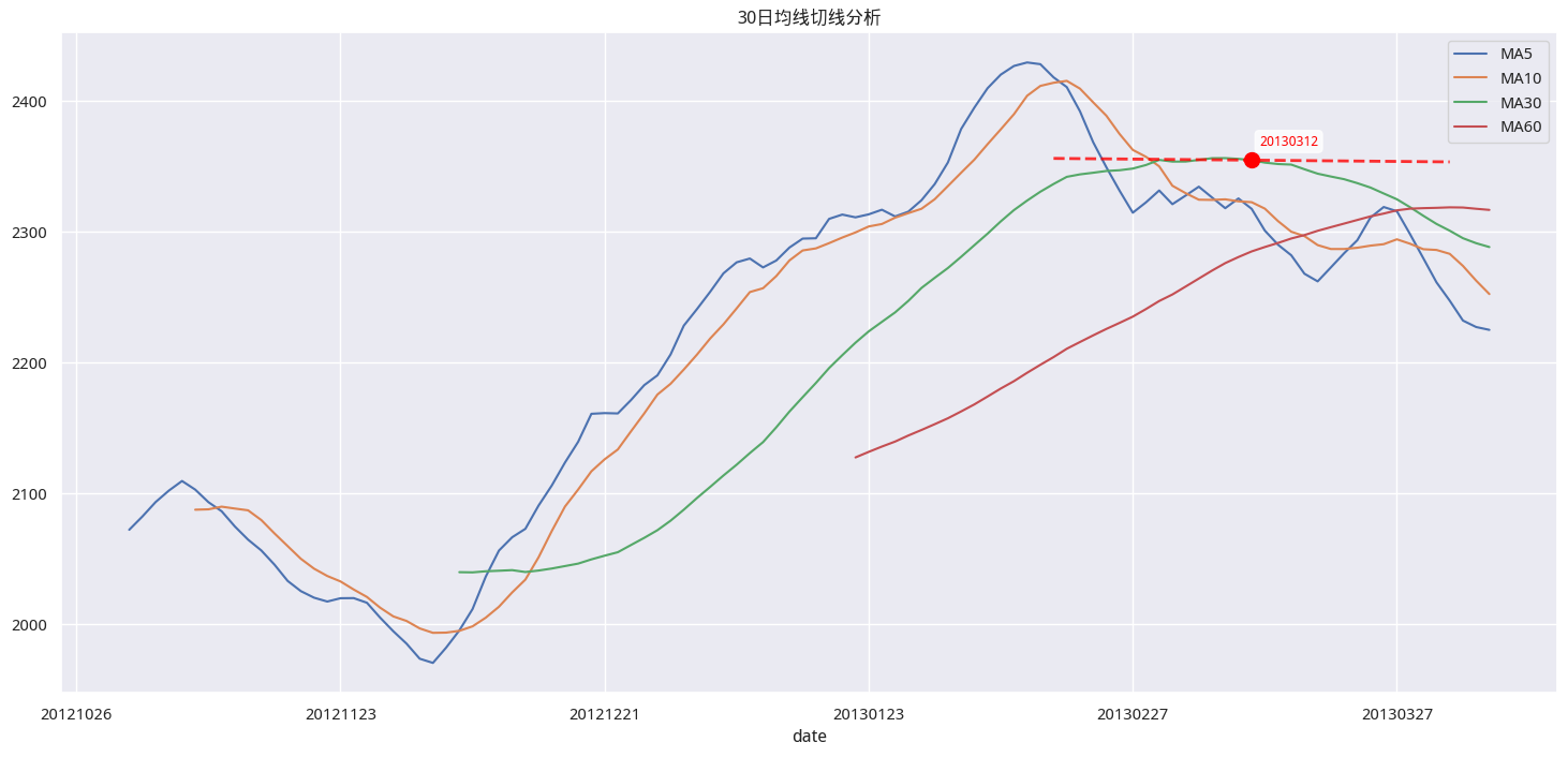
In this chart, the green line represents the 30-day MA. At the red points, the slope of the 30-day MA turns from positive to negative, generating a sell signal. We observe that trend-following using the 30-day MA can capture large swing trades. However, by the time the trendline signals an exit, the price has already dropped significantly from the peak. Conversely, using a shorter-term MA like the 5-day MA generates frequent signals, increasing transaction costs.
This result indicates that traditional MAs suffer from two issues: small windows lead to unsmooth lines and severe jitter in trendline slopes, while large windows result in good smoothness but strong latency.
tip
Identifying tangent reversal points (i.e., when the slope turns from positive to negative, or vice versa) requires some technique. This technique is useful in many contexts: ```python price_df["slope_30_5"] = price_df["slope_30_5"].fillna(0) signs = np.sign(price_df["slope_30_5"]) sign_changes = signs * signs.shift(1) == -1revert_dates = price_df.index[sign_changes]</div>
How can we resolve the inherent trade-off between latency and smoothness in traditional MAs?
## LLT Moving Averages
The research report provides a detailed derivation of the LLT principle. However, understanding LLT requires foundational knowledge such as Z-transforms. We provide a simplified explanation below:
$$\frac{LLT(z)}{price(z)} = \frac{(\alpha-\alpha^2/4) + (\alpha^2/2)z^{-1} - (\alpha-3\alpha^2/4)z^{-2}}{1-2(1-\alpha)z^{-1} + (1-\alpha)^2z^{-2}}$$
This is a formula in the Z-domain, which needs to be transformed into a time-domain formula according to specific rules. The transformation rules are:
- The above equation is the transfer function of a second-order IIR filter. To obtain the time-domain recursive formula, multiply both the numerator and denominator by the denominator's expression, making the denominator 1 (leaving only $LLT(z)$ on the left) and the right side the convolution of the numerator polynomial and $price(z)$:
$$LLT(z) \cdot [1-2(1-\alpha)z^{-1} + (1-\alpha)^2z^{-2}] = price(z) \cdot [(\alpha-\alpha^2/4) + (\alpha^2/2)z^{-1} - (\alpha-3\alpha^2/4)z^{-2}]$$
- After expansion, using the properties of Z-transforms, map $z^{-1}$ and $z^{-2}$ to time-domain periods $t-1$ and $t-2$ respectively:
$$LLT_t - 2(1-\alpha)LLT_{t-1} + (1-\alpha)^2LLT_{t-2} = (\alpha-\alpha^2/4)price_t + (\alpha^2/2)price_{t-1} - (\alpha-3\alpha^2/4)price_{t-2}$$
- Rearrange to obtain the recursive formula:
$$LLT_t = (\alpha-\alpha^2/4)price_t + (\alpha^2/2)price_{t-1} - (\alpha-3\alpha^2/4)price_{t-2} + 2(1-\alpha)LLT_{t-1} - (1-\alpha)^2LLT_{t-2}$$
After transformation, the final formula we obtain is:
$$
y_t = (\alpha-\alpha^2/4)x_t + (\alpha^2/2)x_{t-1} - (\alpha-3\alpha^2/4)x_{t-2} + 2(1-\alpha)y_{t-1} - (1-\alpha)^2y_{t-2}
$$
As seen, the final formula is a recursive function. Here, $y_t$ is the LLT we seek, determined by the previous two LLT values, the most recent three prices, and a parameter $\alpha$.
<!--PAID CONTENT START-->
Its implementation code is:
```python
import numpy as np
import pandas as pd
import matplotlib.pyplot as plt
def calculate_llt(prices, alpha=0.05):
"""
Calculate LLT (Linearly Weighted Least Squares Triangular) Moving Average
Parameters:
prices (array-like): Price sequence
alpha (float): Smoothing coefficient, range (0,1). Smaller values yield smoother lines with more lag.
Returns:
array: LLT moving average sequence
"""
n = len(prices)
llt = np.zeros(n)
# Initialize first two values
if n >= 1:
llt[0] = prices[0]
if n >= 2:
llt[1] = prices[1]
# Calculate coefficients
a1 = alpha - (alpha**2) / 4
a2 = (alpha**2) / 2
a3 = alpha - 3 * (alpha**2) / 4
a4 = 2 * (1 - alpha)
a5 = - (1 - alpha)**2
# Recursively calculate LLT
for t in range(2, n):
llt[t] = a1 * prices[t] + a2 * prices[t-1] - a3 * prices[t-2] + a4 * llt[t-1] + a5 * llt[t-2]
return lltBelow, we compare EMA, the 5-day MA, and the LLT moving average:
price_df = get_price("000001.SH", start, end)
price_df['EMA'] = price_df['close'].ewm(alpha=0.05, adjust=False).mean()
price_df['MA30'] = price_df['close'].rolling(30).mean()
price_df['LLT'] = calculate_llt(price_df['close'], 0.05)
price_df.plot(figsize=(18,8),title='Comparison of Various Trendlines')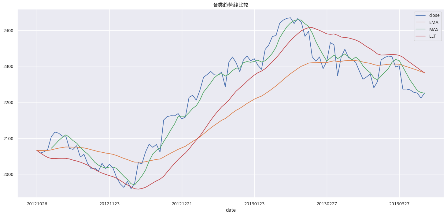
From this single case, LLT indeed tracks more closely (similar to MA5) while achieving relative smoothness (smoother than EMA, similar to MA30).
When calculating LLT, the $\alpha$ parameter affects both smoothness and latency:
for a in [0.03,0.04,0.05]:
price_df[f'LLT(%s)'%a] = calculate_llt(price_df['close'],a)
show_cols = ["LLT(0.03)", "LLT(0.04)", "LLT(0.05)"]
price_df[show_cols].plot(figsize=(18,9),title='LLT Trendlines with Different Alpha Parameters')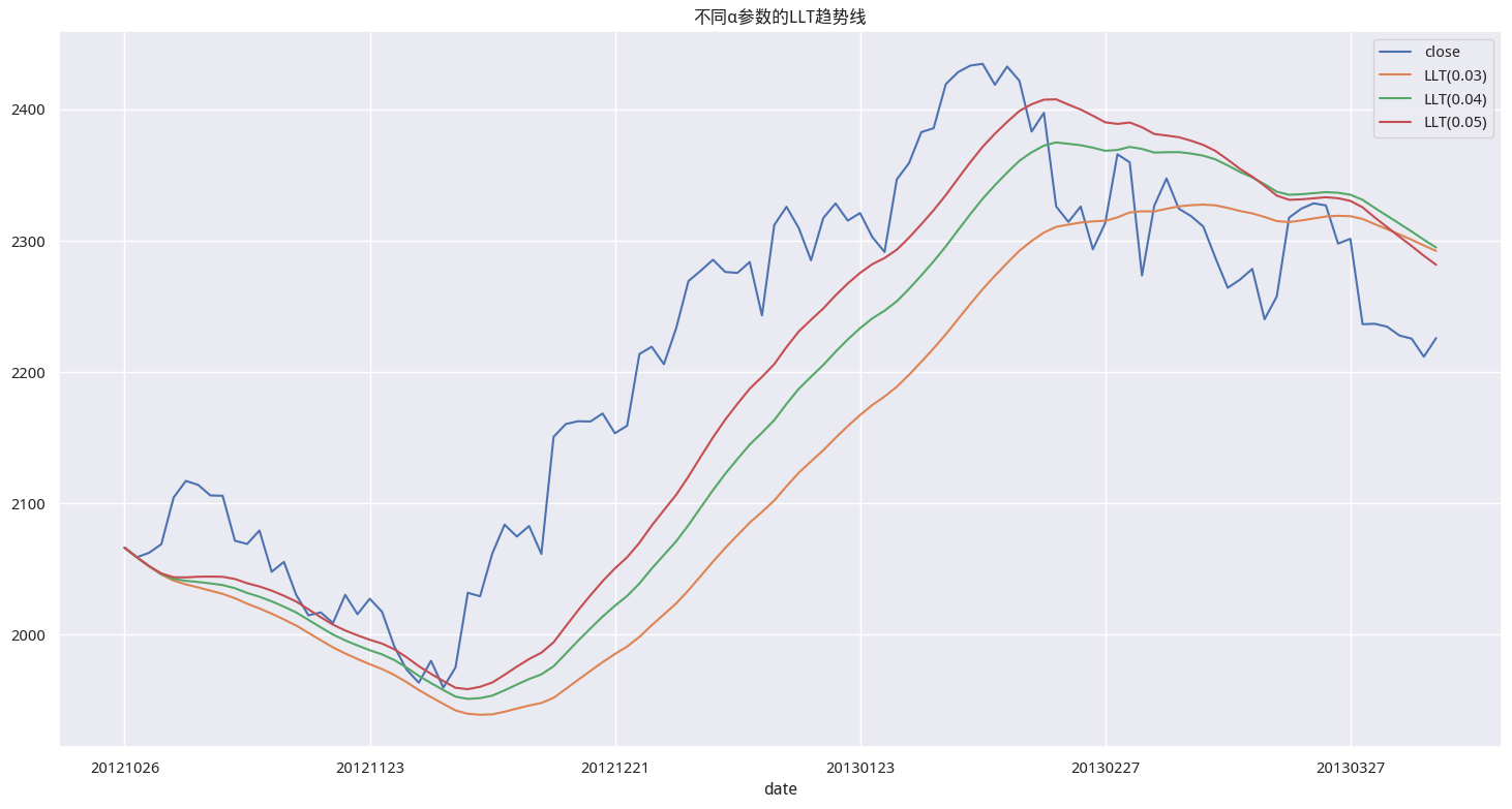
Backtesting and Comparison
First, let's look at the backtest results for traditional MAs. We define a trading function that accepts a dataframe, a factor column name, and the window for slope calculation. We will use the same function for LLT backtesting to ensure a fair comparison.
import quantstats as qs
import quantstats as qs
def trading_strategy(df, factor_col: str, slope_window=5, long_weight=0.5, short_weight=0.5):
"""
Calculate long-short portfolio returns based on MA slope
Parameters:
price_df: DataFrame containing closing prices
factor_col: Factor column name
slope_window: Window size for slope calculation
long_weight: Long position weight (0-1)
short_weight: Short position weight (0-1)
Returns:
DataFrame: DataFrame containing strategy returns
"""
df = df.copy()
df['slope'] = (df[factor_col].rolling(slope_window)
.apply(lambda x: np.polyfit(np.arange(slope_window), x, 1)[0]))
df['signal'] = 0
df.loc[df['slope'] > 0, 'signal'] = 1
df.loc[df['slope'] < 0, 'signal'] = -1
# Calculate daily returns
df['benchmark'] = df['close'].pct_change()
# Calculate long-short portfolio returns
df['long_return'] = np.where(df['signal'] == 1, df['benchmark'], 0)
df['short_return'] = np.where(df['signal'] == -1, -df['benchmark'], 0)
# Portfolio return = Long return * Long weight + Short return * Short weight
df['strategy'] = df['long_return'] * long_weight + df['short_return'] * short_weight
return df
def backtest_ma(start, end, win:int=30):
price_df = get_price("000001.SH", start, end)
factor_col = f"ma{win}"
price_df[factor_col] = price_df["close"].rolling(win).mean()
strategy_df = trading_strategy(price_df, factor_col)
strategy_df.index = pd.to_datetime(strategy_df.index)
qs.plots.returns(
returns=strategy_df["strategy"],
benchmark=strategy_df["benchmark"]
)
metrics = qs.reports.metrics(
returns = strategy_df["strategy"],
benchmark = strategy_df["benchmark"],
display=False
)
print(metrics[:10])
start = datetime.date(2005, 9, 6)
end = datetime.date(2013, 6, 28)
backtest_ma(start, end)Our backtest results on the 30-day MA align with the research report, both showing returns around 300%.
tip
Theoretically