
LLT Strategy Backtest: 25% Annualized or Fatal Flaws?
In the previous article, "Low-Latency Trendlines and Trade Timing," the backtest results for the LLT (Low-Lag Trendline) moving average tangent buy strategy were almost unbelievable. I know you enjoy reading such articles, but few have questioned how credible these results truly are.
This is an opportunity to discuss several critical issues in strategy backtesting. This article reveals the deep technical reasons behind the phenomenon of "backtests buying the earth, live trading losing everything": these issues are hidden within the backtesting framework you use. Unless you examine every detail with a microscope, you might not realize where things are going wrong.
This is also the fundamental reason why quantitative trading can be profitable: the world is essentially a makeshift stage, and not many people are working hard or seriously. If you can efficiently handle every detail, you can outperform anyone.
Disclaimer: This article is published to share how to solve the technical problem of implementing research report strategies in code. Please do not use this as investment advice.
Look-Ahead Bias
In our replication of the research report yesterday, there was actually a hint of using future data. The problem lies in the following code:
df = df.copy()
df['slope'] = (df[factor_col].rolling(slope_window)
.apply(lambda x: np.polyfit(np.arange(slope_window), x, 1)[0]))
df['signal'] = 0
df.loc[df['slope'] > 0, 'signal'] = 1
df.loc[df['slope'] < 0, 'signal'] = -1
# 计算每日收益率
df['benchmark'] = df['close'].pct_change()
# 计算多空组合收益
df['long_return'] = np.where(df['signal'] == 1, df['benchmark'], 0)
df['short_return'] = np.where(df['signal'] == -1, -df['benchmark'], 0)
# 组合收益 = 多头收益 * 多头权重 + 空头收益 * 空头权重
df['strategy'] = df['long_return'] * long_weight + df['short_return'] * short_weight
return dfIf we treat signal as a factor, then in this code, the factor and the forward return are aligned by time, not lagged. That is, the code attributes the return on day $T_0$ to the factor on day $T_0$. However, the exact meaning of the return on $T_0$ is that you must buy on $T_{-1}$ and sell on $T_0$ to calculate it. This is clearly incorrect.
If the stock price rises today, the tangent of the moving average may point upward, resulting in signal = 1; if the stock price falls today, the tangent may point downward, resulting in signal = -1. Both scenarios are unreasonably counted in the portfolio return.
tip
According to the research report, the position building is done as follows:
Although this also has a slight hint of future data, it is allowed in practice because, theoretically, you can calculate the signal and buy during the closing auction: the price used to calculate the signal would not differ much from the final closing price, likely just a slippage difference. Some backtesting tools allow this. For example, backtrader allows buying at the day's closing price if you declare COC (Cheat on Close) to be allowed.
Correcting the Algorithm
Now, let's correct the errors in the above code. Can we also avoid the small flaw of Cheat on Close in the research report?
def backtest(df, calc_signal, args,
price: str = "open",
long_weight: float = 0.5,
short_weight: float = 0.5):
df = df.copy()
df["signal"] = calc_signal(df, *args)
df["signal"] = df["signal"].fillna(0)
df["signal_shifted"] = df["signal"].shift(1)
df["benchmark"] = df[price].pct_change()
df['long_return'] = np.where(df['signal_shifted'] == 1, df['benchmark'], 0)
df['short_return'] = np.where(df['signal_shifted'] == -1, -df['benchmark'], 0)
df["long_short_return"] = df['long_return'] * long_weight + df['short_return'] * short_weight
return dfCompared to the previous version, there are two important differences:
- We shifted the signal back by one row (not forward). Thus, when calculating the position, if the signal from the previous day was 1, we multiply that 1 by the day's return.
- We allow specifying the price data column for calculating returns, defaulting to
open.
If you are familiar with Alphalens, you would know that when calculating returns, it buys at the opening price of the second day after the signal is issued and sells at the opening price of the third day to calculate the return for period = 1D. Now, it seems we are doing exactly that!
The figure below shows the complete process of the first few trades (using synthetic data with fixed alternating gains/losses of 5% and -5%):
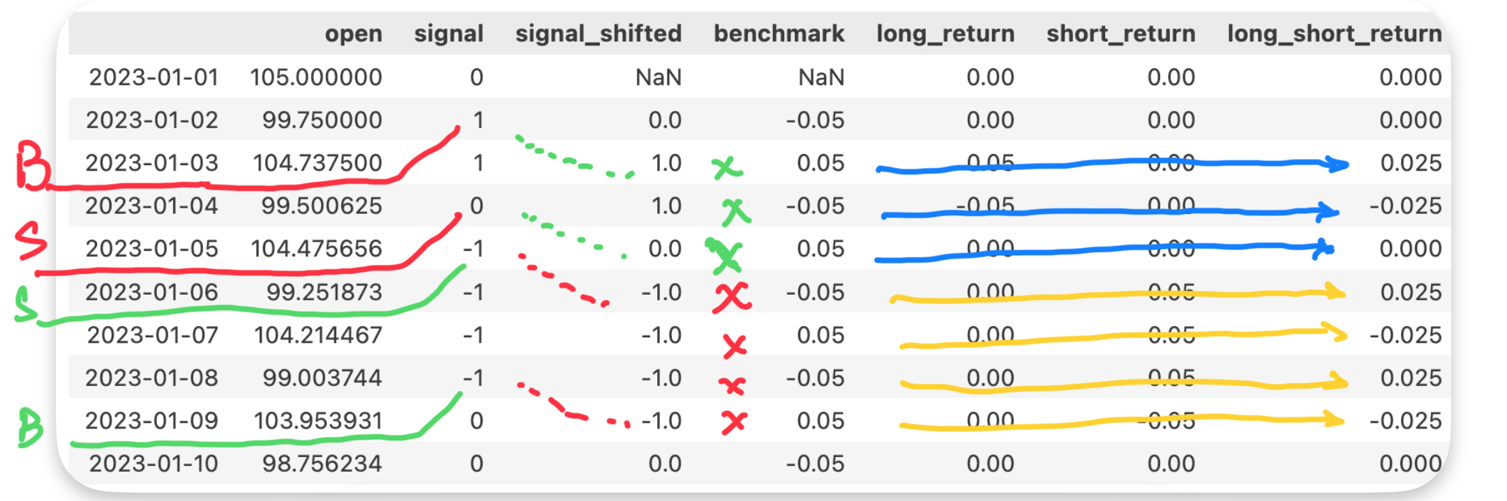
On January 2, the strategy issued a long signal, so we bought long at the open on January 3 at a price of 104.73. With a daily gain of 5%, we used the shifted signal of 1 as the position, resulting in a combined long/short return of 2.5% (assuming 50% position for both long and short). The signal on January 3 was also 1, so we held the position; but since the price dropped 5% that day, the combined return was -2.5%. The signal on the 4th was 0, so the strategy needed to sell at the open on the 5th. On the 5th, since we held no position, the portfolio return was 0.
After using open as the price column for calculating returns, we still get a cumulative return graph almost identical to the previous one. Is this result credible?
It looks correct and perfect. Except for one point: in dataframe-based vectorized backtesting frameworks, we cannot use a strategy that buys at the next day's open. Taking the buy signal on January 2 as an example, since the buy signal (1) on January 2 was shifted to January 3 and counted as a long position, this causes the gain from the January 2 open to the January 3 open to be calculated as long return. However, at the open on January 2, we had not yet executed the long buy.
Considering that if $T_0$ closes with a rise, it is easier to issue a long signal, and the next day's open price is also likely to be higher than the previous day's open, the strategy return calculated this way will have a large component of cheating on the first day. This is the main reason why backtest results look good when returns are calculated using the open price.
But we cannot buy at the open on the third day after the signal is issued (signals don't wait!), so we must use the Cheat on Close strategy, meaning the price column must be specified as "close".
When specifying the price column as close, if we denote the signal occurrence day as $T_0$ and the signal as 1, due to the shift, when calculating the portfolio return on $T_1$, it will be $1 \times T_1$ return. The return on $T_1$ is calculated from the closing price on $T_1$ and the closing price on $T_0$. Although this is a form of Cheat on Close, it does not cause significant error.
The main reason we use DataFrames for backtesting is simplicity and speed. From an idea to live trading, countless processes are involved, taking months (including simulation). Therefore, there is no need to use heavier frameworks at the start. If an idea doesn't work in simple tests, we should probably abandon it -- because statistically, most ideas are invalid anyway.
backtrader: Slower, but More Reliable
For event-driven strategy backtesting, backtrader, although slower, provides more reliable results, as shown by:
backtraderdefaults to buying at the open price on the next bar after the signal is issued.backtradercalculates commissions, position limits, and volume limits.- Vectorized backtesting based on DataFrames is simple, so there is no standard library to implement it. Our manual implementation is prone to errors.
Let's use backtrader to verify the previous backtest results.
The code for calculating LLT and tangent slopes was provided in the previous issue, so it will not be repeated here.
This is the code for calculating llt and tangent slopes to generate signals. Compared to the previous article, we added the thresh parameter, which will be used in tuning.
def calculate_llt(prices, alpha=0.05):
# 转换为numpy数组以避免pandas索引问题
if hasattr(prices, 'values'):
prices = prices.values
n = len(prices)
llt = np.zeros(n)
if n >= 1:
llt[0] = prices[0]
if n >= 2:
llt[1] = prices[1]
a1 = alpha - (alpha**2) / 4
a2 = (alpha**2) / 2
a3 = alpha - 3 * (alpha**2) / 4
a4 = 2 * (1 - alpha)
a5 = - (1 - alpha)**2
for t in range(2, n):
llt[t] = a1 * prices[t] + a2 * prices[t-1] - a3 * prices[t-2] + a4 * llt[t-1] + a5 * llt[t-2]
return llt
# 信号计算函数
def llt_slope_signal(df, d: int=39, slope_window=5, thresh=(0, 0)):
df = df.copy()
alpha = 2 / (d + 1)
df["llt"] = calculate_llt(df["close"], alpha)
df['slope'] = (df["llt"].rolling(slope_window)
.apply(lambda x: np.polyfit(np.arange(slope_window), x, 1)[0]))
signals = pd.Series(0, index=df.index)
signals[df['slope'] > thresh[1]] = 1
signals[df['slope'] < thresh[0]] = -1
signals.ffill(inplace = True)
return signalstip
A note on the parameter `d` for `llt_slope_signal`. It comes from the EMA indicator formula. When `d` takes values like 9, 19, 39, etc., the corresponding alphas are 0.2, 0.1, 0.05, etc.import backtrader as bt
class LLTStrategy(bt.Strategy):
params = (
('d', 39),
('slope_window', 5),
('position_ratio', 1),
('thresh', (0, 0))
)
def __init__(self):
self.order_dict = {}
self.signals = llt_slope_signal(
self.data._dataname,
d=self.p.d,
slope_window=self.p.slope_window,
thresh=self.p.thresh
)
self._last_direction = 0
print(f"策略初始化完成,信号数量: {len(self.signals)}")
print(f"信号前20个值: {self.signals.head(20)}")
def next(self):
current_date = pd.Timestamp(self.data.datetime.date())
current_signal = self.signals.loc[current_date]
position = self.getposition(self.data).size
if current_signal != 0:
print(f"日期: {current_date}, 信号: {current_signal}, 当前持仓: {position}")
if current_signal == 1 and self._last_direction <= 0:
order = self.order_target_percent(target=0.95)
if order:
print(f"做多信号: {current_date.date()}")
elif current_signal == -1 and self._last_direction >= 0:
order = self.order_target_percent(target=-0.95)
if order:
print(f"做空信号: {current_date.date()}")
elif current_signal == 0 and position != 0:
order = self.order_target_percent(target=0.0)
if order:
print(f"平仓信号: {current_date.date()}")
else:
passWe omit the backtest calling code to save space. If you need this code, you can purchase a Quantide membership. If you don't quite understand what we are discussing, you should enroll in Quantide's "Quant 24 Lessons" and "Factor Mining and Machine Learning Strategies."
def run_backtest(data, d=39,
slope_window=5,
thresh=(0,0),
initial_cash=1_000_0000,
commission=1e-4):
cerebro = bt.Cerebro()
cerebro.broker.setcash(initial_cash)
cerebro.broker.setcommission(commission=commission)
cerebro.addstrategy(LLTStrategy, d=d, slope_window=slope_window, thresh=thresh)
bt_data = bt.feeds.PandasData(dataname=data)
cerebro.adddata(bt_data)
# 添加绩效分析器
cerebro.addanalyzer(bt.analyzers.SharpeRatio, _name='sharpe')
cerebro.addanalyzer(bt.analyzers.DrawDown, _name='drawdown')
cerebro.addanalyzer(bt.analyzers.Returns, _name='returns')
# 运行回测
print(f"初始资金: {cerebro.broker.getvalue():.2f}")
results = cerebro.run()
final_value = cerebro.broker.getvalue()
print(f"最终资金: {final_value:.2f}")
# 输出绩效指标
strat = results[0]
returns = strat.analyzers.returns.get_analysis()
sharpe = strat.analyzers.sharpe.get_analysis()
drawdown = strat.analyzers.drawdown.get_analysis()
print(f"夏普比率: {sharpe.get('sharperatio', 0):.2f}")
print(f"最大回撤: {drawdown.get('max', {}).get('drawdown', 0):.2f}%")
print(f"年化收益率: {returns.get('rnorm', 0):.2%}")
return returns.get('rnorm', 0), sharpe.get('sharperatio', 0), drawdown.get('max',{}).get('drawdown',0)
def get_price(symbol, start_date, end_date):
pro = pro_api()
price_df = pro.index_daily(
ts_code=symbol,
start_date=start_date.strftime("%Y%m%d"),
end_date=end_date.strftime("%Y%m%d"),
)
price_df = (
price_df.rename({"trade_date": "date", "ts_code": "asset"}, axis=1)
.sort_values("date", ascending=True)
.set_index("date")
)
price_df.index = pd.to_datetime(price_df.index)
return price_df
start = datetime.date(2005, 9, 6)
end = datetime.date(2013, 6, 28)
prices= get_price("000001.SH", start, end)
run_backtest(prices, commission = 1e-3)The result we obtained was an annualized return of 11.8% and a Sharpe ratio of 0.4. This is slightly better than the benchmark. However, if we backtest the period after 2013, we will find that we have actually just picked up a biting snake:
start = datetime.date(2013, 1, 1)
end = datetime.date(2024, 12, 31)
prices= get_price("000001.SH", start, end)
run_backtest(prices, commission=1e-3)The annualized return this time is -6.4%, with a max drawdown of 79%.
backtrader Parameter Optimization
Should we be disappointed by this?
No! We should never expect a simple strategy, even one with less than 100 lines of code, to become a money-printing machine. Complexity and profundity do not necessarily lead to success, but in capital markets, simplicity or even crudeness is definitely not enough. Any profitable business must have barriers.
Therefore, our optimization journey has just begun. It is far from time to be disappointed!
First, a 0.1% commission fee is too high. When backtesting on indices, we must remember that indices themselves have limited profit space; any leakages are unacceptable!
Currently, most brokerages' trading commissions, especially for quantitative trading, are as low as 0.00854%. So, there is absolutely no need to set such a high commission fee of 0.1%.
info
When we adjusted the commission to 0.01% (still higher than the market), the annualized return improved to -3.7%. That is much better. We will use this setting in subsequent tests. However, this is not strategy optimization. True optimization is about to begin!We decided to use the built-in parameter optimization scheme of backtrader to help us tune. However, tuning may lead to overfitting, so we will also share how to judge whether the tuning results are overfitted.
First, let's define the optimization function.
from IPython.display import clear_output
def optimize(data, d, thresh):
cerebro = bt.Cerebro()
cerebro.broker.setcash(1_000_0000)
# 万分之一的佣金。现在多数券商给到了万分之 0.854
cerebro.broker.setcommission(commission=0.0001)
bt_data = bt.feeds.PandasData(dataname=data)
cerebro.adddata(bt_data)
# 添加绩效分析
cerebro.addanalyzer(bt.analyzers.Returns, _name='returns')
cerebro.optstrategy(LLTStrategy, d = d, thresh = thresh)
strats = cerebro.run(maxcpus = 1, optreturn = True)
clear_output()
params_and_returns = []
for s in strats:
returns = s[0].analyzers.returns.get_analysis()
d, thresh = s[0].params.d, s[0].params.thresh[0]
rnorm, pnl = f"{returns['rnorm']:.2%}", f"{returns['rtot']:.2%}"
params_and_returns.append((d, thresh, rnorm, pnl))
return pd.DataFrame(params_and_returns, columns=["d", "thresh", "rnorm", "pnl"])
start = datetime.date(2008, 1, 1)
end = datetime.date(2012, 12, 31)
prices= get_price("000001.SH", start, end)
result = optimize(prices,
(9, 19, 39, 49, 59),
(
(-0.01, 0.01),
(-0.02, 0.02),
(-0.04, 0.04),
(-0.08, 0.08),
(-0.12, 0.12)
))
resultTo perform parameter optimization via backtrader, the key is these two lines of code:
cerebro.optstrategy(LLTStrategy, d = d, thresh = thresh)
strats = cerebro.run(maxcpus = 1, optreturn = True)When running in a notebook, we must set maxcpus = 1. If maxcpus > 1, it will start multi-process optimization. This involves persisting code in the notebook (because the code needs to be sent to new processes), which will cause errors.
In our "Quant 24 Lessons," we detail how to use backtrader, including strategy optimization.
We let the parameter d take values between (9, 19, 39, 49, 59, 69), corresponding to alphas of (0.2, 0.1, 0.05, 0.03), while thresh takes values between (-0.01, 0.01) and (-0.12, 0.12) in a doubling manner.
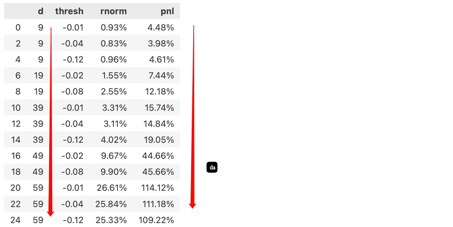 Parameter Optimization
For visual aesthetics, only some results are filtered here.
From the parameter optimization results, d = 59, thresh = -0.01 is the best set, achieving an ultra-high annualized return of 26.6%. Overall, as the d value increases, returns improve; the impact of thresh is not significant. Additionally, there is a parameter affecting performance: how many bars are used to calculate the tangent slope? Here, only a fixed 5 were used.
The above parameter optimization was based on data from 2008 to 2012. How does it perform between 2005 and 2013? The conclusion is: the annualized return reached 25.6%.
If we use these parameters for investment from 2013 to 2014, we will get an annualized return of 13.9% and a Sharpe ratio of 0.97. This result is quite good.
Correctly Viewing Overfitting
When using backtrader for parameter optimization, we must be aware that overfitting is more likely to occur.
In the previous section, we already applied the optimal parameters obtained based on [2008, 2012] to the past [2005, 2012] and future [2013, 2014] periods to compare the results. This is a method to test for overfitting. If parameters are not overfitted, they should tell a good story on data they have not seen before.
Here is another approach regarding the thresh parameter. Based on thresh to determine signal is obviously more reasonable than simply judging signal based on 0, which is beyond doubt. But will the optimized thresh parameter lead to overfitting? At this point, we can observe the distribution of tangent slopes:
def llt_slope(df, d: int=59, slope_window=5):
df = df.copy()
alpha = 2 / (d + 1)
df["llt"] = calculate_llt(df["close"], alpha)
df['slope'] = (df["llt"].rolling(slope_window)
.apply(lambda x: np.polyfit(np.arange(slope_window), x, 1)[0]))
return df['slope']
start = datetime.date(2005, 1, 1)
end = datetime.date(2013, 12, 31)
prices= get_price("000001.SH", start, end)
slopes = llt_slope(prices, d = 39)
slopes.plot(kind='hist')
s1 = (slopes < -0.02).sum()/len(slopes)
s2 = (slopes < 0.02).sum()/len(slopes)
s2 - s1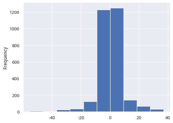 Tangent Slope Distribution
It can be seen that by setting thresh to [-0.02, 0.02], we only excluded about 0.3% of the data. This indicates: we did not use hacking methods to exclude most scenarios, leaving only a small amount of data that makes the final returns look good. Therefore, at least for the thresh parameter, it is very likely that overfitting has not occurred here.
If we use the parameters d = 59, thresh = [-0.01, 0.1] optimized from the 2008-2012 data unchanged for 2013 to 2024, the annualized return will decay to 2.79%. This shows that market styles are constantly changing. This strategy is essentially a $\beta$ factor.
However, we can update the parameters every few years and then use this strategy for a short period thereafter.
The following code demonstrates how to search for optimized parameters based on the past 5 years of data and then use them for investment in the subsequent two years:
rolling_results = []
for year in range(2014, 2026, 2):
opt_start = datetime.date(year - 6, 1, 1)
opt_end = datetime.date(year - 1, 12, 31)
prices = get_price("000001.SH", opt_start, opt_end)
result = optimize(
prices,
(19, 39, 49, 59),
((-0.01, 0.01), (-0.02, 0.02), (-0.04, 0.04), (-0.08, 0.08), (-0.12, 0.12)),
)
clear_output()
# 找出最佳参数
result["cagr"] = result.rnorm.str.strip("%").astype(float)
max_row = result[result.cagr == result.cagr.max()]
d, thresh = max_row[["d", "thresh"]].values[0].tolist()
# 对接下来的两年进行回测
backtest_start = datetime.date(year, 1, 1)
backtest_end = datetime.date(year + 1, 12, 31)
prices = get_price("000001.SH", backtest_start, backtest_end)
returns, sharpe, drawdown = run_backtest(prices, d = d, thresh = (thresh, -1 * thresh))
rolling_results.append([
year, year + 1, d, thresh, f"{returns:.2%}", sharpe, f"{drawdown:.2f}%"
])
clear_output()
# 运行时间较长,因此我们在一次运行之后中断。
break
columns=["start", "end", "d", "thresh", "returns", "sharpe", "drawdown"]
pd.DataFrame(rolling_results, columns=columns)Finally, we obtained the annual (two-year) returns as follows:
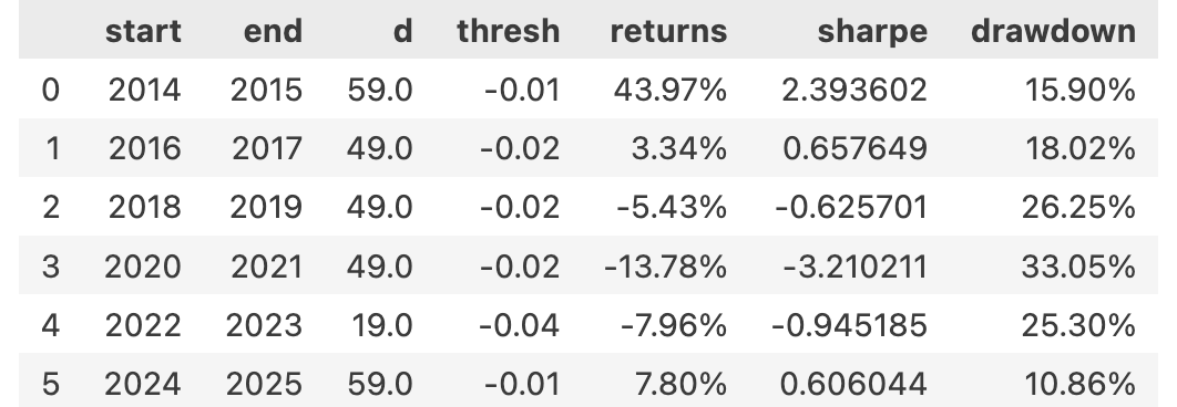
If we shorten the validation period (e.g., changing the strategy run time from two years to 1.5 years after parameter optimization), this strategy still brought good returns from 2023 to 2025. You can try changing the parameters and running it yourself.