
RSRS Timing Factor: Backtest, Replication, and Alpha Analysis
The RSRS factor, applied to the CSI 500 index from March 2005 to March 2017, yielded a total return of 1432.36% over 12 years, with an annualized return of 24.84% and a Sharpe ratio of 1.42. In contrast, the benchmark index returned only 290.13% during the same period.
The core idea is to treat the daily high and low prices as resistance and support levels, respectively, and use the slope of a linear regression fitted over a given period as the factor. A steeper slope indicates stronger market momentum.
This notebook reproduces the RSRS factor. The complete, runnable code and data are available on our research platform. If you are interested in its latest performance or performance over any specific period, you can simply adjust the time parameters to obtain the results.
The RSRS (Resistance Support Relative Strength) factor is a timing factor proposed by Everbright Securities in a series of research reports starting in 2017. The series was initially published in 2017, with subsequent reviews and optimizations of the factor construction in 2019 and 2021. This notebook reproduces this factor and interprets its construction logic.
This is one of our series of research report interpretations. By following this series, you will master the theoretical knowledge, programming skills, data acquisition methods, and trading strategy experience required to replicate research reports—in short, becoming a proficient strategy researcher.
When interpreting each research report, we attach the original report:
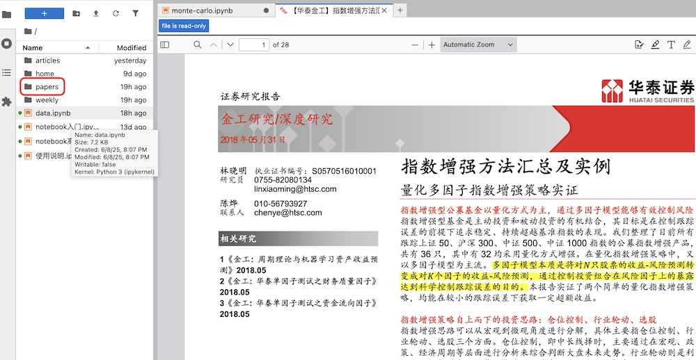
Followed by our interpretation and replication:
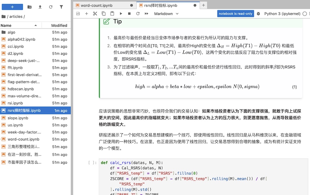
By comparing the two, you will find that we have refined and mined the research report, making the theme clearer and easier to understand.
The main idea of this strategy is:
tip
1. The daily high and low prices represent the true resistance and support derived from the博弈 (game/interaction) of all market participants. 2. Between two adjacent time points $[T_0, T_1]$, the ratio of the change in the high price $\Delta_H = High(T_1) - High(T_0)$ to the change in the low price $\Delta_L = Low(T_1) - Low(T_0)$ reflects the relative strength of resistance versus support, which is the RSRS indicator. 3. To filter noise, we generally perform linear regression on the high and low prices over $T_1, T_2, ..., T_n$. The resulting slope $\beta$ is the RSRS indicator, which is essentially the same as Definition 2, expressed by the following formula:$$ high = alpha + beta * low + epsilon, \quad epsilon \sim N(0, sigma) $$
The research report authors also hand-drew two figures to illustrate this idea:
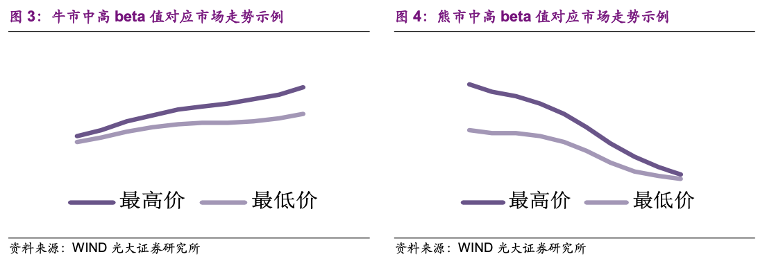
The report also demonstrates a simple but common technique for modeling trading ideas: linear regression. Since Tinbergen et al. pioneered econometrics, linear regression has been widely used in economic and financial fields. Here, the introduction of linear regression allows for a reasonable abstraction of the trading idea into a model supported by statistical evidence.
The calculation method for this factor is as follows:
import pandas as pd
def calc_rsrs_factor(df: pd.DataFrame, win: int = 18):
df = df.copy()
# 计算滑动窗口的协方差 Cov(low, high)
rolling_cov = df["low"].rolling(window=win).cov(df["high"])
# 计算滑动窗口的方差 Var(low)
rolling_var = df["low"].rolling(window=win).var()
df["RSRS"] = rolling_cov / rolling_var
return df["RSRS"]tip
Here, we use a fast vectorized algorithm. If you find this algorithm difficult to understand, its vanilla version is as follows: ```python def calc_rsrs_vanilla(df, N): df = df.copy() temp = [np.nan] * N for row in range(len(df) - N):
y = df['high'][row : row + N]
x = df['low'][row : row + N]
# Ensure x and y have length N and no NaN values
if len(x) == N and len(y) == N and not x.isnull().any() and not y.isnull().any():
beta = np.polyfit(x, y, 1)[0]
temp.append(beta)
else:
temp.append(np.nan)
df['rsrs'] = temp
return df</div>
In comparative testing, if the vanilla version takes 4.3ms, the vectorized version takes only 317us—more than 10 times faster.
Now, using data from Tushare, let’s look at the factor calculation results. The following code shows how to retrieve HS300 index data:
```python
pro = ts.pro_api()
hs300 = pro.index_daily(ts_code = "000300.SH", start_date = "20250101", end_date = "20250601")
hs300.index = pd.to_datetime(hs300["trade_date"])
hs300 = hs300.sort_index(ascending=True)tip
When using Tushare’s market data, please ensure you set `trade_date` as the index and sort the data as shown in the code snippet. This ensures the data order matches that of most software systems.hs300_factor = calc_rsrs_factor(hs300, 18)
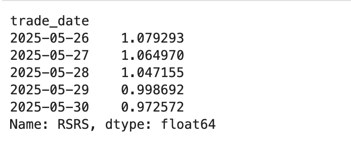
hs300_factorWe see that hs300_factor is a pd.Series with dates as the index and factor values as the data. This format is convenient for merging cross-sectional data later.
How is the factor’s quality? We can use Alphalens for testing. Alphalens is a library for evaluating factors, simple and easy to use, making it ideal for quick factor assessment. However, it primarily uses cross-sectional evaluation. Therefore, we need to first obtain historical data for all constituent stocks of the CSI 300 index and calculate their factor values.
tip
Read many research reports but don’t know how to replicate them? In 2025, you should join the Kuangti Research Platform, which guides you step-by-step in replicating research reports. For just 360 RMB per year, you gain access to over 100 research reports, replication code, and the runtime environment! This environment includes an advanced Tushare account (official price 500 RMB), which alone justifies the cost!In our research environment, we have daily historical data for all individual stocks from 2005 to 2023, allowing for long-cycle factor testing. We also have an encapsulated alpha_test method available for use. However, we still need to obtain the list of CSI 300 constituent stocks.
df = pro.index_weight(
index_code='000300.SH',
start_date='20231201',
end_date='20231231'
)
# 在研究环境中,我们使用的股票代码是以。XSHG 或者。XSHE 结尾的,所以,我们需要将股票代码转换一下。
def convert_symbol(x: str):
if x.endswith(".SH"):
return x.replace(".SH", ".XSHG")
elif x.endswith(".SZ"):
return x.replace(".SZ", ".XSHE")
else:
raise ValueError(f"{x}: not supported format")
universe = tuple(map(convert_symbol, df["con_code"].unique()))
universe[:5]Now, we call alphatest to perform factor testing:
start = datetime.date(2018, 1, 1)
end = datetime.date(2021, 12, 31)
_ = alphatest(universe, start, end, calc_rsrs_factor)The output results were somewhat unexpected. There was no high return as anticipated; in fact, the annualized Alpha was negative. However, we must view Alphalens’ output dialectically. This simple test already indicates that the factor likely possesses Alpha (its beta is close to zero), but the annualized return is negative. In this case, simply reversing the factor’s direction yields a positive annualized return.
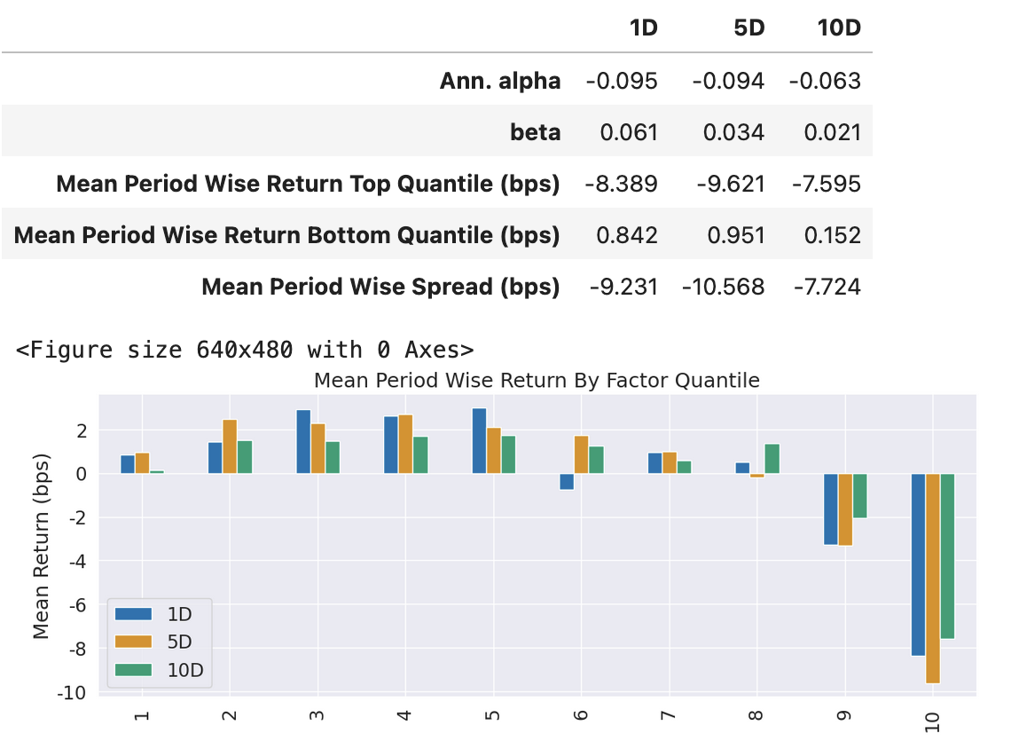
However, the Alphatest results differ significantly from the research report. How should this be explained?
It turns out that the trading method for the RSRS indicator in the research report is threshold-based buy/sell. It requires stratified statistics of the slope factor over the past M trading days, taking the mean ± one standard deviation as the buy and sell thresholds. Thus, this is an event-driven trading method, which Alphalens cannot accurately backtest for returns.
tip
Alphalens’ default backtesting method is cross-sectional. Although event-driven backtesting was added later, support is incomplete. Perhaps considering that backtesting frameworks already have mature event-driven mechanisms, they didn’t invest much effort here? With Quantopian’s dissolution, we can no longer know the reasons.The alphatest here is an auxiliary function we developed in our Factor Analysis and Machine Learning Strategy course. It calls Alphalens’ backtesting functions at the底层 (lower level) but simplifies them, allowing us to complete factor backtesting with just one line of code.
Now, let’s return to the research report’s implementation and backtest trading directly on the CSI 300 index itself.
Event-driven trading strategies must provide trading signals. Based on the previous discussion, this signal is one standard deviation from the mean. To this end, we first need to statistically analyze the RSRS over the past M days, calculate the mean and standard deviation, and then perform z-score normalization.
However, before starting, let’s visualize the factor to get a feel for it.
import seaborn as sns
import matplotlib.pyplot as plt
import numpy as np
import scipy.stats as st
def describe(df, col, title):
data = df[~df[col].isna()][col]
# 创建图形
fig, axes = plt.subplots(1, 2, figsize=(18, 9))
plt.suptitle(title)
# 基本统计量
avg = data.mean()
std = data.std()
# 左侧:直方图
sns.histplot(data, kde=False, stat='density', alpha=0.4, ax=axes[0])
for line, color, label in zip(
[avg, avg-std, avg+std],
['red', 'blue', 'blue'],
['Mean', '-1 Standard Deviation', '1 Standard Deviation']
):
axes[0].axvline(x=line, color=color, linestyle='--', linewidth=0.8, label=label)
axes[0].set_ylabel('Percentage', fontsize=10)
axes[0].legend(fontsize=12)
# 右侧:KDE 和正态分布拟合
x = np.linspace(avg - 3*std, avg + 3*std, 100)
kde = st.gaussian_kde(data)
y_norm = st.norm.pdf(x, avg, std)
axes[1].plot(x, kde(x), label='Kernel Density Estimation')
axes[1].plot(x, y_norm, color='black', linewidth=1, label='Normal Fit')
axes[1].axvline(x=avg, color='red', linestyle='--', linewidth=0.8, label='Mean')
axes[1].set_ylabel('Probability', fontsize=10)
axes[1].legend(fontsize=12)
return plt.show()
# 调用函数
describe(hs300_factor.to_frame(), 'RSRS', '2018-2025 斜率数据分布')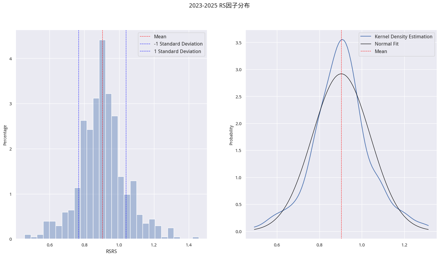 Slope Data Distribution
According to the research report and running results, the sell threshold is around 0.8, and the buy threshold is around 1.0. That is, if the RSRS indicator is greater than 1.0, buy and hold; when RSRS drops below 0.8, sell.
If we determine thresholds based on this, we would commit look-ahead bias: we included all data from 2023 to 2025 in the statistics. But what if trading occurred at the end of 2023? Unless the distribution of RSRS has remained unchanged over these years, we would definitely be referencing incorrect thresholds.
Therefore, we need to determine trading thresholds using a sliding window. That is, within $T_0 ~ T_m$ trading days, find the 25th and 75th percentiles to serve as the buy or sell thresholds for day m. In the research report, it uses another method: z-score normalization of the N-day regression slope of high on low across win windows. After z-score normalization, if the factor value on a given day is greater than 0.7, it is considered a buy signal; if less than -0.7, it is a sell signal.
info
In a standard normal distribution, the value 0.7 corresponds to the 75.8th percentile, and -0.7 corresponds to the 24.9th percentile. The research report did not strictly follow the previously mentioned ±1 standard deviation, likely to align with common percentiles like 25% and 75%.start = "20180101"
end = "20250601"
hs300 = pro.index_daily(ts_code = "000300.SH", start_date = start, end_date = end)
hs300.index = pd.to_datetime(hs300["trade_date"])
hs300 = hs300.sort_index(ascending=True)
def calc_rsrs(df: pd.DataFrame, win: int = 18):
df = df.copy()
# 计算滑动窗口的协方差 Cov(low, high)
rolling_cov = df["low"].rolling(window=win).cov(df["high"])
# 计算滑动窗口的方差 Var(low)
rolling_var = df["low"].rolling(window=win).var()
df["rsrs"] = rolling_cov / rolling_var
return df
def calc_rsrs_zscored(df: pd.DataFrame, n: int = 18, m: int = 600):
df = calc_rsrs(df, n)
df["rsrs_"] = df["rsrs"].fillna(0)
ZSCORE = (df['rsrs_'] - df['rsrs_'].rolling(m).mean()) / df['rsrs_'].rolling(m).std()
df['rsrs_z'] = ZSCORE
return df.drop(columns='rsrs_')
rsrs_z = calc_rsrs_zscored(hs300, 18, 600)We can observe the z-score normalized factor:
describe(rsrs_z, 'rsrs_z', '2018-2025 Z-Score 化后的 RSRS 分布')The results are not significantly different from the previous figure (Slope Data Distribution), so they are omitted here.
Now, let’s construct a simple trading strategy:
import matplotlib.dates as mdate
def RSRS_Strategy(start: datetime.date, end: datetime.date, n: int=18, m: int=600):
start_ = start.strftime("%Y%m%d")
end_ = end.strftime("%Y%m%d")
data = pro.index_daily(ts_code = "000300.SH", start_date = start_, end_date = end_)
data.index = pd.to_datetime(data["trade_date"])
df = data.sort_index(ascending=True)
rsrs_z = calc_rsrs_zscored(df, n, m) # 计算标准分指标
# 需要扣除前期计算的 600 日
rsrs_z=rsrs_z[max(n, m):]
print('回测起始日:',min(rsrs_z.index))
z_singal = []
threshold = 0.7
for row in range(len(rsrs_z)):
if rsrs_z['rsrs_z'][row] > threshold:
z_singal.append(1)
else:
if row != 0:
if z_singal[-1] and rsrs_z['rsrs_z'][row] > -threshold:
z_singal.append(1)
else:
z_singal.append(0)
else:
z_singal.append(0)
# 交易信号
rsrs_z['z_singal'] = z_singal
# 每日收益
rsrs_z['ret'] = rsrs_z['close'].pct_change()
# 累积净值
z_cum = (1+rsrs_z['z_singal']*rsrs_z['ret']).cumprod()
# 基准净值
benchmark = (1+rsrs_z['ret']).cumprod()
# 画图
plt.figure()
fig = plt.figure(figsize=(20, 10))
ax1 = fig.add_subplot(1, 1, 1)
ax1.plot(z_cum, label='RSRS 策略')
ax1.plot(benchmark, label='沪深 300')
ax1.xaxis.set_major_formatter(mdate.DateFormatter('%Y-%m'))
plt.legend(loc='best')
plt.xlabel('时间')
plt.ylabel('净值')
plt.title('RSRS 指标策略净值曲线')
plt.show()
return z_cum, benchmark
strategy, benchmark = RSRS_Strategy(
datetime.date(2005, 1, 1), datetime.date(2018, 1, 1), m=300
)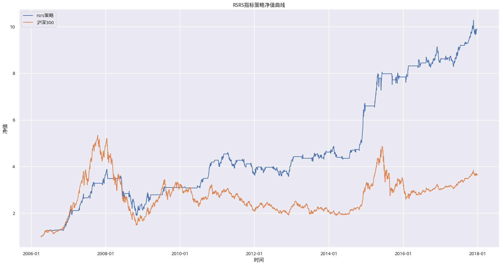
The research report was published in 2017. We used 11 years of data from 2005 to 2018 for backtesting. From the simple net value curve, the strategy, with a 10-fold increase, far exceeded the benchmark model, closely matching the research report’s results.
Part of the code in this article references Hugo2046’s GitHub project. Special thanks are extended.